【论文笔记】A Meta-Reinforcement Learning Algorithm for Causal Discovery

标题：针对元强化学习的因果发现算法。

Abstract

Causal discovery is a major task with the utmost importance for machine learning since causal structures can enable models to go beyond pure correlation-based inference and significantly boost their performance.
因果发现是机器学习的一项最重要的主要任务，因为因果结构可以使模型超越纯粹的基于相关性的推理，并显著提高它们的性能。

However, finding causal structures from data poses a signifi-cant challenge both in computational effort and accuracy, let alone its impossibility without interventions in general.
然而，从数据中寻找因果结构在计算努力和准确性方面都是一个重大的挑战，更不用说没有一般干预的不可能了。

1. develop a meta-reinforcement learning algorithm that performs causal discovery by learning to perform interventions such that it can construct an explicit causal graph.
   开发一种元强化学习算法，通过学习执行干预来执行因果发现，这样它就可以构建一个明确的因果图。
2. the estimated causal graph also provides an explanation for the data-generating process.
   估计的因果图也为数据生成过程提供了一个解释。
3. our algorithm estimates a good graph compared to the SOTA approaches, even in environments whose underlying causal structure is previously unseen.
   与SOTA方法相比，我们的算法估计了一个很好的图，即使在潜在因果结构以前未见的环境中。
4. make an ablation study that shows how learning interventions contribute to the overall performance of our approach.
   做一项消融研究，显示学习干预如何有助于我们的方法的整体表现。

1 MOTIVATION AND CONTRIBUTION

As solving such a task requires strong generalisation and transfer (of knowledge) skills, it also stands as one of the challenges with utmost importance in machine learning (ML) research.
由于解决此类任务需要强大的概括和**（知识）转移**技能，因此它也是机器学习（ML）研究中最重要的挑战之一。

Causal discovery is the task of finding the true causal structure of an environment, given some data of observable variables in the environment. These structures enable models to go beyond pure correlation-based inference and significantly boost their performance.
因果发现的任务是在给定环境中可观察变量的一些数据的情况下，找到环境的真实因果结构。这些结构使模型能够超越纯粹的基于相关性的推理，并显著提高其性能。

很多学者在因果关系的ML上有进展，但是ML也推动了因果关系的出结论

To infer causal structure from data it has been shown that it is necessary to perform interventions; that is to experimentally ‘force’ a variable to take on a certain value.
为了从数据中推断因果结构，已经证明有必要进行干预，即通过实验“迫使”一个变量能够具有一定的值。

Only these interventions allow us to, in general, distinguish causal structures which yield the same distribution over their variables.
一般来说，只有这些干预措施才允许我们区分对其变量产生相同分布的因果结构。

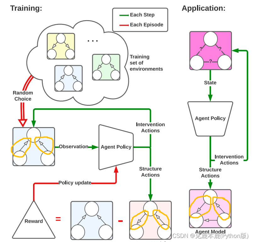
In this article, we develop a meta-learning algorithm in a reinforcement learning (RL) setting where the agent learns to perform interventions to construct a causal graph.
在本文中，我们开发了一个在强化学习(RL)设置中的元学习算法，在其中智能体学习执行干预来构建一个因果图。

因果发现算法的一些举例：

模型	内容
Constraint-based algorithms	infer the causal relationships through independence tests on purely observational data.
Score-based algorithms	incrementally add and delete edges such that the structure of the causal model is improved w.r.t. a scoring function.（增量添加和删除边，使因果关系的结构模型采用改进的w.r.t.评分函数。）
search over the space of permutations rather than a graph space（在排列空间上进行搜索，而不是在图空间上进行搜索）	with extensions even to soft interventions

Rather, using RL, it solves a prediction task that depends on the ability of the model to learn causal effects from interventions in the environment.
解决一个预测任务，从环境的干预中得到因果关系。

Almost all aforementioned approaches can not make use of interventions at all or are computationally inefficient.
几乎所有上述方法都根本不能充分利用干预措施，或者计算效率低下。

This is largely due to their inability to use previous information to generalise to unseen environments.
这在很大程度上是因为他们无法使用以前的信息来概括到看不见的环境。

With these considerations in mind, our main contributions tackle some of the common issues found in causal discovery, briefly formulated as follows.
解决因果发现问题中的比较普遍的问题。

1. computationally efficient use of interventions;
   计算上高效使用干预措施
2. generalization to environments with unseen causal structure;
   推广到具有看不见的因果结构的环境（提升泛化性）

2 PRELIMINARIES AND NOTATION

Causal relationships are formally expressed in terms of a structural causal model (SCM), and every SCM induces a graph structure $G$ in which each node and edge represent a random variable and direct causal effect between nodes, respectively.

1. 使用结构化的因果模型（SCM）；
2. 每个SCM包含一个图结构 $G$ ；
3. 每个 $G$ 包含节点和边界，节点表示随机变量，边界表示直接因果关系；

We define an SCM $S$ as a tuple $(\chi ,\mu ,\psi ,\rho )$
用一个元组数据表示SCM的一个状态$(\chi ,\mu ,\psi ,\rho )$

where χ = { χ 1 , ⋯   , χ ∣ χ ∣ } \chi= \{ \chi_{1}, \cdots, \chi_{|\chi|} \} χ={ χ1​,⋯,χ∣χ∣​} is the set of observable (also called endogenous) variables;
$\chi$是可观测集，也称作内在集

μ = { μ 1 , ⋯   , μ ∣ μ ∣ } \mu = \{\mu_{1}, \cdots, \mu_{|\mu|} \} μ={ μ1​,⋯,μ∣μ∣​} is the set of unobservable (also called exogenous) variables;
$\mu$是不可观测集，也称作外在集

ψ = { ψ 1 , ⋯   , ψ ∣ ψ ∣ } \psi = \{\psi_{1}, \cdots, \psi_{|\psi|}\} ψ={ ψ1​,⋯,ψ∣ψ∣​}is the set of functions whose elements are defined as structural equations in the form of ${\chi }_i\leftarrow f_i(P{a}_{Xi}^G,U_i)$ in which $P{a}_{Xi}^G$ is the set of observable parents of $X_i$ w.r.t. $G$;
$\psi$其元素被定义为结构方程的函数集

P = { P 1 , ⋯   , P ∣ μ ∣ } P = \{P_{1}, \cdots, P_{|\mu|}\} P={ P1​,⋯,P∣μ∣​} is a set of pairwise independent distributions where $U_i\sim P_i$.
$U_i\sim P_i$是成对形式的独立分布

Moreover, we will assume that unobservable variables do not have any parents in $G$ i.e., every $U_i$ is a root node.
不可观测的变量没有父节点，也就是每个不可观测的$U_i$都是一个根节点

We will assume the induced causal graph is always a directed acyclic graph (DAG) i.e., acyclic SCM.
我们假设诱导因果图总是一个有向无环图(DAG)，即无环SCCM。

We will also make use of the notion of a partially directed acyclic graph (PDAG) which can be thought of as a DAG where some edges are relaxed to be bi-directional, and cyclicity is only limited to those edges (in other words, one cannot obtain a cycle only by using uni-directional edges).
我们假设诱导因果图总是一个有向无环图(DAG)，即无环SCM。
我们也将利用部分有向无环图(PDAG)的概念。PDAG可以被认为是一个DAG，一些边放松是双向的，和循环只局限于这些边（换句话说，不能只通过使用单向边获得一个循环）。

A intervention on a variable ${\chi }_i$ is defined as the action of replacing the corresponding structural equation ${\chi }_i\leftarrow f_i(P{a}_{Xi}^G,U_i)$ with ${\chi }_i\leftarrow x$ for some value $x$, which we simply denote as $\mathbf{do}({\chi }_i=x)$.
对变量的干预被定义为替换相应的结构方程的作用

This makes the intervened variable (causally) independent of its parents, changing the causal mechanism behind the data-generation process.
这使得干预变量（因果地）独立于其父母，改变了数据生成过程背后的因果机制。

The model is causal in the sense that one can derive the distribution of a subset ${\chi }^{\prime }\subseteq \chi$ of variables following an intervention on a set of variables, also called intervention target, $I\subseteq \chi /{\chi }^{\prime }$.
该模型是因果关系，因为人们可以在对一组变量进行干预后，得出变量的子集${\chi }^{\prime }\subseteq \chi$的分布，也称为干预目标，$I\subseteq \chi /{\chi }^{\prime }$。

We call the resulting distribution over $\chi$ the post-interventional distribution.
我们将$\chi$上的结果分布称为介入后分布。

Accordingly, the purely observational case will be denoted as empty intervention i.e., $I=\varnothing$, without any change to the causal structure whatsoever
因此，纯观察性的情况将被表示为空干预，即I=∅，而对因果结构没有任何改变。

3 WORKING ASSUMPTIONS

1. Each environment is defined by an acyclic SCM.
   每个环境都由一个无环SCM定义。
2. Every observable variable can be intervened on.
   每个可观察到的变量都可以被干预。
3. For each environment in the training set, the underlying SCM is given.
   训练集给出潜在的SCM。
4. For all intervention targets $I$, ∣ I ∣ ∈ { 0 , 1 } |I| \in \{0, 1\} ∣I∣∈{ 0,1} (i.e., we are performing interventions on at most one variable at a time.)
   一次最多只对一个变量进行干预。

4 REINFORCEMENT LEARNING SETUP

4.1 ACTIONS

两种离散动作。
第一种类型是对环境进行干预，并观察变量的结果值。我们将把这种行为称为倾听行动（listening action）。

All, except for one, of the listening actions are intervention actions that intervene on exactly one variable (i.e. $|I|=1$).
除了一个人之外，所有的倾听行动都是只干预一个变量的干预行动

还有一个附加的倾听行动，我们称之为非行动。
当采取非动作时，智能体会观察可观测变量的当前值，而不进行干预(即，$I=\varnothing$)。
这一行动解释了纯粹的观测数据的收集。

第二种类型的行动负责构建环境因果结构的认知模型，这是目前对主体的最佳(PDAG)估计。
我们将把这些动作称为结构-动作。
每个结构行为都可以添加、删除或逆转认知因果模型的一个边缘。

对于一个有$n$个节点的图，有$n(n-1)$可能的边，因此有$3n(n-1)$的结构作用。
连同倾听动作，我们有$2n+1+3n(n-1)=3n^2-n+1$动作。
动作空间的大小是节点大小的二次型。
当将删除或反向操作应用于当前模型中不存在的边时，将忽略该操作。这实际上相当于执行非操作。
当添加动作应用于已经在认知模型中的边缘时，情况同样成立。

4.2 STATE SPACE

The state of the environment consists of a concatenation of three parts.
状态空间是三个部分的拼接。

1. The first one encodes the current values of the $n$ observable variables.
   第一个部分编码了当前的可观测状态；
2. The second part is a one-hot encoding of which variable is currently being intervened on.
   第二个部分是对正在进行干预的变量的独热编码；
3. The third part of the state encodes the current epistemic model as a vector.
   第三个将当前的认识模型编码成了向量；

Each value of this vector represents an undirected edge in the graph. The edges in the vector are ordered lexicographically（有序的词汇学）.

1. The value $0$ encodes that there is no edge between the two nodes.
2. The value $0.5$ encodes that there is an edge going from the lexicographically smaller node to the bigger node of the undirected edge. （逻辑意义上小的节点向大的节点链接。）
3. The value $1$ encodes that there is an edge in the opposite direction.

4.3 REWARDS AND EPISODES

One obvious choice is to count the edge differences between the two graphs. This ensures that generating a model that has more edges in common with the true DAG will be preferred over one which has fewer edges in common.
一个明显的选择是计算这两个图之间的边差。这确保了生成一个与真正的DAG有更多共同边的模型。

It further gives a strong focus on causal discovery as opposed to scores based on causal inference.
它进一步强调了因果发现，而不是基于因果推理的分数。

The Structural Hamming Distance (SHD) provides a metric that describes a way of counting the differences between two directed graphs.
结构汉明距离(SHD)提供了一种度量，描述了一种计算两个有向图之间的差异的方法。

In our case, it takes two PDAGs and counts how many of the following operations are needed to transform the first PDAG into the second: add or delete an undirected edge, and add, remove, or reverse the orientation of an edge.
在我们的例子中，它需要两个PDAG，并计算将第一个PDAG转换为第二个PDAG需要多少以下操作：添加或删除一条无向边，以及添加、删除或反转一条边的方向。

For implementational purposes we adapt this metric to not count reverse actions as such but by counting them as add and delete actions instead. Further, we count undirected edges as bi-directed edges. This results in a metric that simply counts the distinguishing edges of two directed graphs.
为了实现目的，我们调整这个度量以不计算反向操作，而是将它们计算为添加和删除操作。此外，我们将无向边计算为双向边。这就产生了一个度量来计算两个有向图的有区别边的数量。

Given a predicted directed graph $S_p=(V,E_P)$ and a target, directed graph $S_T=(V,E_T)$, we define the dSHD as $$dSHD(E_P,E_T)=|\frac{E_P}{E_T}|+|\frac{E_T}{E_P}|$$.

As we need to determine when the estimation of the model terminates, we set a finite horizon $H$ for each episode.
由于我们需要确定模型的估计何时终止，我们为每个情节设置了一个有限的视野$H$。

The estimation of the epistemic model is complete when $H-1$ actions were taken.
当采取了$H-1$个动作之后，认知模型的估计完成。

Note that when a small episode length is chosen, there might not be enough steps available to the agent to collect enough data and make the right changes to the epistemic model.
请注意，当选择小情节长度时，智能体可能没有足够的步骤来收集足够的数据并对认知模型进行正确的更改。

We suggest that the episode length should be at least $n+\frac{n(n-1)}{2}$, which allows for one intervention on each node and one operation per possible edge in the graph.
我们建议剧集长度至少应该是$n+\frac{n(n-1)}{2}$，这允许对每个节点进行一次干预，并在图中的每个可能边缘进行一次操作。

Further, $H$ should not be set too large since additional learning complexity might be introduced.
此外，H不应该设置得太大，因为可能会引入额外的学习复杂性。

At the beginning of each episode, an SCM is sampled from the training set. The epistemic causal model of the agent is reset to a random PDAG, to further introduce randomness.
在每集开始时，从训练集中采样SCM。代理的认知因果模型重置为随机PDAG，以进一步引入随机性。

The evaluation is done by calculating the negative $dSHD$ between the generated PDAG and the true causal graph only at the end of each episode. Every other step receives a reward of $0$.
评估是通过仅在每个事件结束时计算生成的PDAG和真实因果图之间的负$dSHD$来完成的。每隔一步获得$0$的奖励。

$${\mathbf{V}}_{\pi }(s)={\mathbf{E}}_{\pi }[-{\gamma }^H\mathbf{dSHD}(edges(s_H),E_{Env})|s_t=s]$$
where

1. $edges(s)$ is the operator that returns the edges of a state;
   返回状态边缘的操作函数
2. $E_{Env}$ are the edges of the current target graph;
3. $H\in N$ is the horizon;
4. $\gamma$ is the discount factor $\gamma \in [0,1]$;

We use the Actor-Critic with Experience Replay algorithm to solve this RL problem.
We choose this algorithm because it sets a good balance between sample-efficient off-policy methods and its (potential) easy extension to continuous action spaces.
我们选择该算法是因为它在样本有效的非策略方法和其（潜在的）易于扩展到连续动作空间之间建立了良好的平衡。

We use a discount factor $\gamma =0.99$ and a buffer size of $500000$. All other parameters are according to the standard values of the Python library we used (Stable-Baselines 2.10.1).

4.4 POLICY NETWORK

Our policy has a fully-connected feed-forward actor network and a fully connected feed-forward critic network. Both networks are preceded by a shared network that has n fully-connected feed-forward layers followed by a single LSTM layer.
我们的策略有一个完全连接的前馈参与者网络和一个完全连接的前馈批评者网络。
这两个网络之前都有一个共享网络，该网络有$n$个完全连接的前馈层，后跟一个LSTM层。

The exact amounts of layers and their sizes are specified for each experiment.
其他的部分随实验而异

We want to emphasise the recurrent LSTM layer. It enables the policy to memorize past information of its preceding layers and, therefore, use information from previous observations. More specifically, it should enable the policy to remember samples from the (post-interventional) distributions induced by the data-generating SCM earlier in that episode.
LSTM层使策略能够记住其前一层的过去信息，因此，使用以前观察到的信息。
更具体地说，它应该使策略能够记住该episode早期数据生成SCM引起的（介入后）分布中的样本。

We argue that this should help to better identify causal relations since the results of sequential interventions can be used to estimate the distribution.
我们认为，这应该有助于更好地识别因果关系，因为顺序干预的结果可以用来估计分布。

5 LEARNING TO INTERVENE

First, we develop a toy example to test whether our approach can learn to perform the right interventions to identify causal models under optimal conditions.
首先，我们开发了一个玩具示例，以测试我们的方法是否可以学习在最佳条件下执行正确的干预来识别因果模型。

To this end, we construct a simple experiment in which two observationally equivalent, yet interventionally different environments have to be distinguished.
为此，我们构建了一个简单的实验，在该实验中，必须区分两个在观测上等效但在干预上不同的环境。

Thus, if our policy learns to distinguish those environments, it has to learn to perform interventions.
因此，如果我们的策略学会了区分这些环境，它就必须学会进行干预。

The two environments are governed by the fully observable, 3-variable SCMs with structures $G_1$ : $X_1\leftarrow X_0\to X_2$ and $G_2$ : $X_0\to X_1\to X_2$.
全观测的、三变量的SCMs

In both environments, the root node $X_0$ follows a normal distribution with $X_0\sim N(\mu =0,\sigma =0.1)$. The nodes $X_1$ and $X_2$ take the values of their parents in the corresponding graph.
根节点服从正态分布，其他的两个节点都从相应的图中获得数值

The resulting observational distributions $P_{G_1}(X_0,X_1,X_2)$ and $P_{G_2}(X_0,X_1,X_2)$ are the same and so are the post-interventional distributions after interventions on $X_0$ or $X_2$.

For an intervention on $X_1$, $P_{G_1}(X_0,X_2|\mathbf{do}(X_1=x))\ne P_{G_2}(X_0,X_2|\mathbf{do}(X_1=x))$. Hence the two SCMs can only be distinquished by intervening on $X_1$.

During training, we observe that the mean $dSHD$ of the produced graphs is 0.0 with a standard derivation of 0.0. This is a perfect reproduction of the two environments in all cases. This indicates that our policy has learned to use the right interventions to find the true causal structure.
在训练期间，我们观察到生成的图的平均dSHD为0.0，标准差为0.0。这在所有情况下都是两种环境的完美再现。这表明我们的政策已经学会了使用正确的干预措施来找到真正的因果结构。

After training, we apply the converged policy 10 times to each of the environments and qualitatively analyze the behaviour.
训练后，我们将收敛策略应用于每个环境10次，并定性分析行为。

What the resulting 20 episodes have in common is that, towards the beginning of each episode, they tend to delete edges that do not overlap in the two environments.
由此产生的20集的共同点是，在每集开始时，它们往往会删除在两种环境中不重叠的边缘。

Then an intervention on X1 is performed. Depending on the outcome of the intervention, either $G_1$ or $G_2$ is ultimately generated.
然后对$X_1$进行干预。根据干预的结果，$G_1$或$G_2$是最终生成。这也可以在示例中看到。

1. 学习的策略学会了使用$X_1$的干预来区分这两种环境。
2. 能够逐步使用干预措施来进行因果发现。
3. 已经学会了只执行相关的干预措施，而不是随机干预措施。

6 GENERALISATION OF CAUSAL KNOWLEDGE

Given a structure $G$ with a set of observable variables $\chi$, we model our environments as $\forall X\in \chi$
$$X\leftarrow \left(\sum _{Y\in P{a}_X^G}WY\right)+ϵ$$

创建了24个包含3个可观察变量的SCMs和542个包含4个可观察变量的SCMs。这些集合中的SCMs都诱导了不同的因果结构。我们将把在测试集上表现最好的模型称为最佳模型。

We created a random baseline that returns a random DAG.
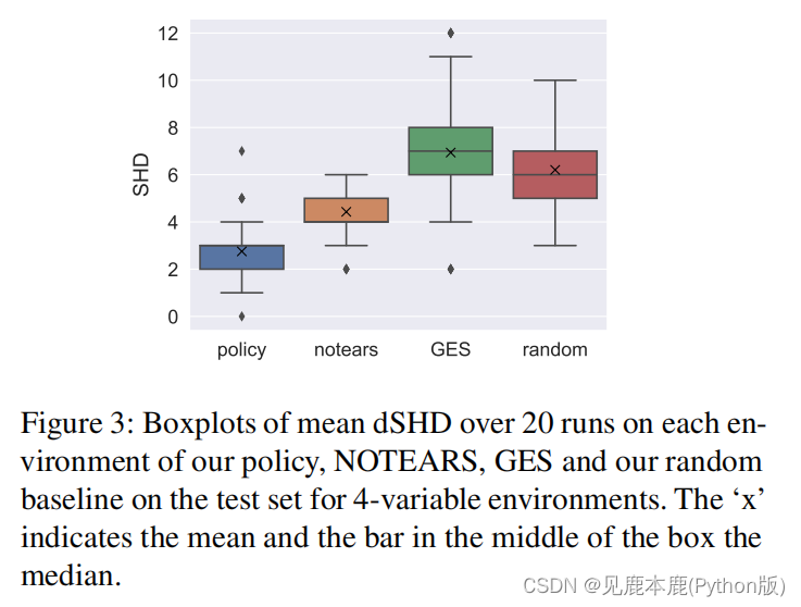
To compare the learned policies to other state-of-the-art approaches, we ran our best model and the other approaches (NOTEARS [Zheng et al., 2018, 2020], GES [Chickering, 2002, Kalainathan and Goudet, 2019], random) 20 times on each of the environments in the test sets and computed the directed SHD for each of the generated graphs.
我们创建了一个返回一个随机DAG的随机基线。
比较学习的策略与其他先进的方法，我们运行我们最好的模型和其他方法20次在每个环境测试集和计算每个生成的图的定向SHD。

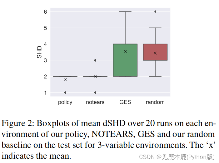
Our policy outperforms the GES algorithm which is based on purely observational data.
本文策略优于基于纯观测数据的GES算法。

This also suggests that our model can generalise to previously unseen environments.
这也表明，我们的模型可以推广到以前从未见过的环境中。

One possible explanation is that the quality gain w.r.t. NOTEARS and GES is attributed to the fact that they are both based on purely observational
data, whereas our policy leverages interventional data.
一种可能的解释是，质量增益为w.r.t.无眼泪和GES归因于它们都是基于纯粹的观察数据，而我们的政策利用了干预数据。

7 CONTRIBUTION OF INTERVENTIONS

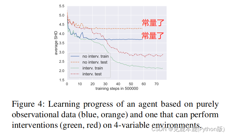
We train a variant of our policy which is based on purely observational data (we disallow the use of interventions) and compare it to the model which uses interventions.
我们训练了一种基于纯粹的观察性数据的策略变体（我们不允许使用干预措施），并将其与使用干预措施的模型进行比较。

We can see in the first part, that the average dSHD on the test and training of both models compares similarly.
在第一部分中我们可以看到，两个模型的测试和训练上的平均dSHD比较相似。

What stands out is that after approximately 10 million training steps, the performance of the model without interventions turns out to be approximately constant.
值得注意的是，经过大约1000万步的训练后，没有干预的模型的表现被证明是近似恒定的。

At about the same amount of training steps, the model which uses interventions starts to rapidly perform better until reaching almost 30 million training steps in total.
在大约相同数量的训练步骤下，使用干预措施的模型开始迅速表现得更好，直到总共达到近3000万个训练步骤。

For the model with interventions, a learning process emerges with two fast learning regions. We argue that this behavior emerges from a two-phase learning process. First, the model learns to produce a graph, based on purely observational data. And then, they learn to use interventions (if enabled) to further increase performance.

1. 该模型学习了如何基于纯粹的观测数据来生成一个图。
2. 学会了使用干预措施（如果能够实现）来进一步提高性能。

Ultimately, in the 4-variable environments, our model outperforms NOTEARS no matter whether it uses interventional data or purely observational one. Nonetheless, the model using interventional data outperforms the one using purely observational data. Overall, these empirical results support the idea that interventions help to identify causal structures from data.
最终，在4变量环境中，无论我们的模型是使用介入数据还是纯观察数据，其性能都优于NOTEARS。尽管如此，使用介入数据的模型还是优于使用纯观测数据的模型。总的来说，这些实证结果支持了干预措施有助于从数据中识别因果结构的观点。

8 DISCUSSION AND CONCLUSION

9 ACKNOWLEDGEMENTS