论文阅读 | Border-Peeling Clustering

Abstract—In this paper, we present a novel non-parametric clustering technique. Our technique is based on the notion that each latent cluster is comprised of layers that surround its core, where the external layers, or border points, implicitly separate the clusters. Unlike previous techniques, such as DBSCAN, where the cores of the clusters are defined directly by their densities, here the latent cores are revealed by a progressive peeling of the border points. Analyzing the density of the local neighborhoods allows identifying the border points and associating them with points of inner layers. We show that the peeling process adapts to the local densities and characteristics to successfully separate adjacent clusters (of possibly different densities). We extensively tested our technique on large sets of labeled data, including high-dimensional datasets of deep features that were trained by a convolutional neural network. We show that our technique is competitive to other state-of-the-art non-parametric methods using a fixed set of parameters throughout the experiments.

摘要-本文提出了一种新的非参数聚类技术。我们的技术基于这样一个概念，即每个潜在的簇都是由围绕其核心的层组成的，外部层或边界点隐含地将簇分开。与以前的技术不同，比如DBSCAN，在DBSCAN中，团簇的核心是由密度直接定义的，在这里，潜在的核心是通过边界点的渐进剥离来揭示的。通过分析局部邻域的密度，可以识别边界点并将其与内层的点相关联。我们证明，剥离过程适应于局部密度和特性，成功地分离出相邻的团簇（可能密度不同）。我们在大量的标记数据上广泛地测试了我们的技术，包括由卷积神经网络训练的深层特征的高维数据集。在整个实验过程中，我们使用了五组固定的参数，证明了我们的技术与其他最先进的非参数方法是有竞争力的。

Index Terms—Clustering, non-parametric techniques

关键词-聚类，非参数技术

1 INTRODUCTION

CLUSTERING is the task of categorizing data points into groups, or clusters, with each cluster representing a different characteristic or similarity between the data points. Clustering is a fundamental data analysis tool, and as such has abundant applications in different fields of science and is especially essential in an unsupervised learning scenario. Ideally, a clustering method should infer the structure of the data, e.g., the number of clusters, without any manual supervision.

聚类是将数据点分类为组或簇的任务，每个簇表示数据点之间的不同特征或相似性。聚类是一种基本的数据分析工具，因此在不同的科学领域有着广泛的应用，在无监督的学习场景中尤为重要。理想情况下，聚类方法应该推断数据的结构，例如，聚类的数量，而不需要任何人工监督。

​ Many of the state-of-the-art clustering methods operate with several underlying assumptions regarding the structure of the data. A prominent assumption is that the clusters have a single area that can be identified as the center, or the core of the cluster. For instance, K-Means [1] operates under the assumption that there is a single cluster center according to the compactness of the data, while the Mean-Shift [2] method defines this area as the one displaying the highest density inside the cluster. Operating under this assumption may result in overly split clusters containing several dense areas, or centers, of smaller clusters.

许多最先进的聚类方法都是基于数据结构的一些基本假设。一个突出的假设是，簇只有一个区域，可以确定为簇的中心或核心。例如，K-Means[1]根据数据的紧凑性假设存在单个聚类中心，而Mean-Shift[2]方法将该区域定义为显示聚类内部最高密度的区域。在这种假设下运行可能会导致过度分裂的簇，其中包含几个较小簇的密集区域或中心。

​ Density based methods like DBSCAN [3] operate often under the assumptions that different clusters have similar levels of density, and that the cores of the clusters can be defined based on density reasoning. However, often, the cores of the clusters do not have a clear structural density that can be directly defined, leading to a redundant merge of adjacent clusters.

像DBSCAN[3]这样基于密度的方法通常是在假设不同的簇具有相似的密度水平的情况下操作的，并且可以基于密度推理来定义簇的核心。然而，通常情况下，簇的核心没有清晰的结构密度可以直接定义，导致相邻簇的冗余合并。

​ In this work, we introduce Border-Peeling: a non-parametric clustering method that iteratively peels off layers of points to reveal the cores of the latent clusters. The peeling is a local process, where the decisions are a result of local analysis, revealing the local behaviour of points without expecting other clusters to share similar characteristics. Our technique is non-parametric in the sense that the number of clusters is not provided as input. The careful repeated peeling forms a transitive association between the peeled border points and the remaining core points. The key is to consider a layered structure for the latent clusters, where the external layers implicitly separate the clusters. We analyze the density of the local neighborhoods of each point to iteratively estimate the border points and associate them with inner-layer points. See Fig. 1 for an illustration our iterative technique.

在这项工作中，我们介绍了边界剥离：一种非参数聚类方法，迭代剥离点层，以揭示潜在聚类的核心。剥离是一个局部过程，决策是局部分析的结果，揭示了点的局部行为，而不期望其他簇具有相似的特征。我们的技术是非参数化的，因为簇的数目不是作为输入提供的。仔细的重复剥离在剥离的边界点和剩余的核心点之间形成了一个传递关联。关键是考虑潜在簇的分层结构，其中外部层隐含地分离簇。我们分析每个点的局部邻域密度，迭代估计边界点并将其与内层点关联。关于我们的迭代技术，请参见图1。

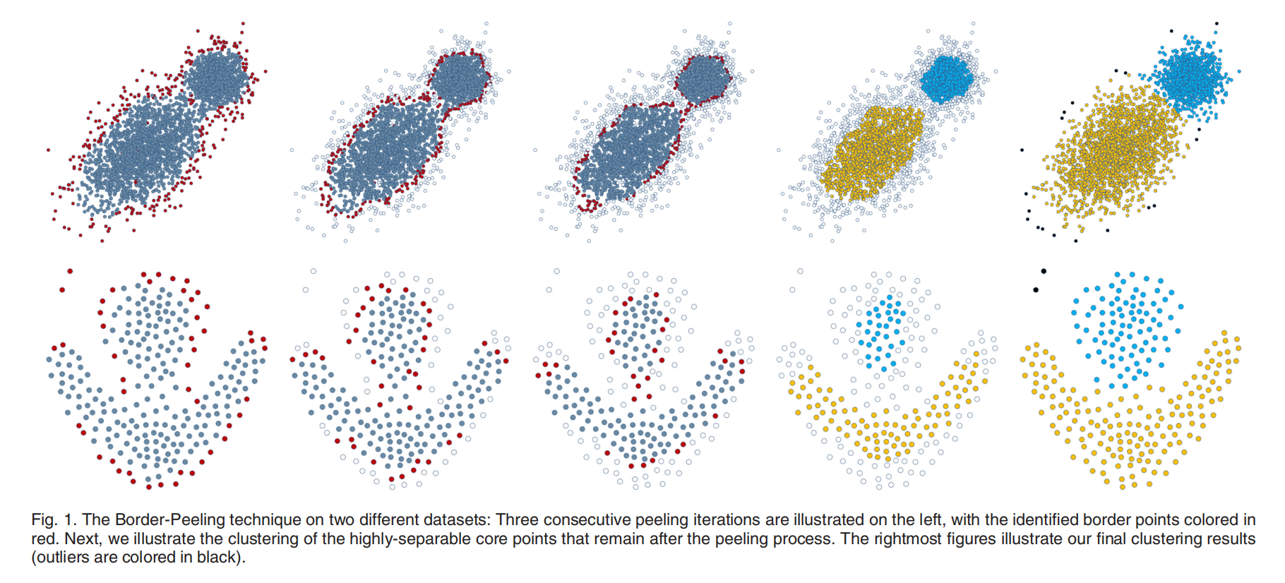
图1 两个不同数据集上的边界剥离技术：三个连续的剥离迭代在左侧显示，已识别的边界点用彩色表示红色。接下来，我们将说明剥离过程后保留的高度可分离的核心点的聚类。最右边的数字说明了我们最终的聚类结果（异常值用黑色表示）。

​ In the following sections, we describe the details of our method, and demonstrate the performance of our method on various datasets and in comparison to other well-known clustering methods. Except for common baseline datasets, we use large datasets, containing thousands of points, for which we have their ground truth clusters, and extensively evaluated the performance using many random subsets. Particularly, we evaluate our technique on high-dimensional datasets of deep features that were trained by convolutional neural networks. We show that the Border-Peeling clustering algorithm is competitive to other state-of-the-art non-parametric clustering methods using a fixed set of parameters throughout the experiments.

在下面的部分中，我们将详细描述我们的方法，并演示我们的方法在各种数据集上的性能，并与其他著名的聚类方法进行比较。除了常见的基线数据集外，我们使用包含数千个点的大型数据集，这些数据集具有基本的真值聚类，并使用许多随机子集广泛地评估性能。特别是，我们评估了我们的技术在高维数据集的深层特征是由卷积神经网络训练。在整个实验过程中，我们使用五个固定的参数集证明了边界剥离聚类算法与其他最先进的非参数聚类方法是有竞争力的。

2 RELATED WORK

Data clustering is one of the most fundamental problems in data analysis, highly applicable to various fields of science. For a comprehensive survey on data clustering techniques, please refer to [4]. In our work, we present a novel non-parametric clustering method. Non-parametric clustering is an active fifield of research, receiving ongoing attention for several decades now. In what follows, we elaborate on the most closely related works.

数据聚类是数据分析中最基本的问题之一，非常适用于各个科学领域。有关数据聚类技术的全面综述，请参阅[4]。在我们的工作中，我们提出了一种新的非参数聚类方法。非参数聚类是一个非常活跃的研究领域，几十年来一直受到人们的关注。接下来，我们将详细介绍最密切相关的研究。

​ The DBSCAN [3] method groups together points that are packed together closely , marking points that lie individually in low-density regions as noise. The notion of border points within a cluster has been established by DBSCAN in the past. The border points in DBSCAN are defifined as points that are part of a cluster but are not surrounded by a dense neighborhood. A notable difference between their method and ours is that in DBSCAN, the identifified border points do not have a prominent role in the defifinition of the different clusters. Furthermore, the association to their resulting cluster is dependent on the order in which they are processed. Additionally, the DBSCAN method has been shown to be sensitive to its input parameters [5]. Later works, e.g., [6], [7], extended their work to allow for an automatic parameter estimation.

DBSCAN[3]方法将紧密堆积在一起的点分组，将单独位于低密度区域的点标记为噪声。簇内边界点的概念在过去由DBSCAN建立。DBSCAN中的边界点被定义为簇的一部分，但不被密集邻域包围。他们的方法和我们的方法的一个显著区别是，在DBSCAN中，已识别的边界点在不同簇的定义中没有显著的作用。此外，与它们产生的簇的关联取决于它们被处理的顺序。此外，DBSCAN方法对其输入参数非常敏感[5]。后来的工作，如[6]，[7]，扩展了他们的工作，允许自动参数估计。

​ The OPTICS [8] clustering technique extends DBSCAN. Unlike DBSCAN, it can detect clusters in data of varying density by producing a reachability plot with an ordering of the data points according to their clusters. However, OPTICS requires a manual analysis of the reachability plot. Furthermore, it does not have a notion of border points. HDBSCAN [9], a recent extension of both DBSCAN and OPTICS, is a hierarchical version of DBSCAN, where a flat partition, consisting of the most prominent clusters, can be extracted from the hierarchy. HDBSCAN only requires one parameter (the minimum cluster size) and can handle data of varying density. Similarly to OPTICS, HDBSCAN does not have a notion of border points. However, due to the fact that HDBSCAN chooses the density threshold automatically, by comparing hierarchies of dense areas, it tends to cluster a large number of data points as noise.

OPTICS(Ordering points to identify the clustering structure)[8]聚类方法扩展了DBSCAN。与DBSCAN不同的是，它可以通过生成一个可达图来检测不同密度数据中的簇，并根据簇对数据点进行排序。然而，OPTICS需要手动分析可达性图。此外，它没有边界点的概念。HDBSCAN[9]是DBSCAN和OPTICS的最新扩展，是DBSCAN的分层版本，其中可以从分层中提取由最突出的簇组成的平面分区。HDBSCAN只需要一个参数（最小集群大小），可以处理不同密度的数据。与OPTICS类似，HDBSCAN没有边界点的概念。然而，由于HDBSCAN自动选择密度阈值，通过比较密集区域的层次结构，往往会将大量的数据点作为噪声进行聚类。

​ CHAMELEON [5] is a hierarchical method of clustering, which partitions the data according to its k-NN graph and merges the components of the graph according to their proximity and inter-connectivity. However, as discussed in [10], this method may yield sub-optimal results for data in higher dimensions. Other more recent hierarchical methods have been shown to effectively handle outlier points [11], [12]. The work presented in [10] suggests a clustering technique based on a shared (mutual) nearest neighbor (SNN) approach. It has been shown that such an approach is advantageous when the goal is to fifind the most signifificant clusters, rather than identifying all the latent clusters [13].

CHAMELEON[5]是一种分层聚类方法，它根据数据的k-NN图对数据进行划分，并根据数据的邻近性和连通性对数据进行合并。然而，正如[10]中所讨论的，这种方法可能会对高维数据产生次优结果。其他较新的分层方法已被证明能有效地处理离群点[11]，[12]。文献[10]提出了一种基于共享（相互）最近邻（SNN）方法的聚类技术。已经证明，当目标是找到最重要的聚类，而不是识别所有潜在的聚类时，这种方法是有利的[13]。

​ The Mean-Shift [2] method clusters data points using a kernel density estimation function, by iteratively shifting each data point to a dense region in its proximity, and then clustering the shifted data points. It is, however, dependent on the bandwidth parameter of the kernel density estimator. The Adaptive Mean-Shift [14] method overcomes this issue by estimating a different bandwidth for each data point according to the local neighborhood of the point. As mentioned in [15], in many cases, Mean-Shift clustering tends to over-partition the clusters, i.e., it often returns a large number of clusters, even when the actual number of clusters is small. In our work, over-partitioning is avoided due to our peeling termination criterion, which is determined automatically according to the characteristics of the data.

Mean-Shift[2]方法使用核密度估计函数对数据点进行聚类，通过迭代地将每个数据点移动到其附近的密集区域，然后对移动的数据点进行聚类。然而，它依赖于核密度估计器的带宽参数。自适应Mean-Shift[14]方法通过根据每个数据点的局部邻域估计不同的带宽来克服这个问题。如[15]所述，在许多情况下，均值漂移聚类往往会过度划分聚类，即它通常会返回大量聚类，即使实际聚类数很小。在我们的工作中，由于剥离终止准则是根据数据的特征自动确定的，因此避免了过度划分。

​ The Affinity Propagation [16] technique clusters data points according to the concept of message passing between data points. Affinity propagation performs the clustering by first finding exemplars in the dataset, and then clustering each data point according to the exemplar that the data point was associated with. Our method also uses data point association to cluster the data points. However, unlike our method, Affinity Propagation tends to overpartition the data.

近邻传播聚类算法（AP）根据数据点之间消息传递的概念对数据点进行聚类。近邻传播聚类通过首先在数据集中找到样本来执行聚类，然后根据数据点关联的样本对每个数据点进行聚类。该方法还利用数据点关联对数据点进行聚类。然而，与我们的方法不同，近邻传播聚类倾向于过度分配数据。

​ The topic of identifying cluster border points was previously addressed in Xia et al. [17], where the points in the datasets are ordered according to the number of k-neighborhoods in which they participate (Reverse KNN), and points with a low number of neighborhoods are considered to be the border points. In their work, the border identification is presented as a general pre-processing step which may improve the clustering result. However, they do not address to the issue of classifying the points to different clusters, as well as to the clustering itself. The QCC algorithm [18] bears some similarity to our method as it also utilizes reverse k-nearest neighbors, however, conceptually, it is quite different. Unlike our method where the cluster borders are iteratively peeled, QCC is a center-based approach, where the clustering results are driven by the estimated cluster centers.

在Xia等人[17]中，先前讨论了识别簇边界点的话题，其中数据集中的点根据其参与的k-邻域的数量排序（反向KNN），邻域数量较少的点被认为是边界点。在他们的工作中，边界识别作为一个一般的预处理步骤，可以提高聚类结果。但是，它们并没有解决将点分类到不同聚类以及聚类本身的问题。QCC算法[18]与我们的方法有一些相似之处，因为它也使用了反向k-近邻，然而，在概念上，它是完全不同的。与我们的方法不同，QCC是一种基于中心的方法，聚类结果由估计的聚类中心驱动。

3 THE ALGORITHM

​ Given a set of points in ${\mathbb{R}}^d$, our clustering technique iteratively peels off border points from the set. The premise of this method is that by repeatedly peeling off border points, the final remaining points, termed core points will be better separated and easy to cluster.

给定$ \mathbb {R} ^ d $中的一组点，我们的聚类技术会从集合中迭代剥离边界点。 此方法的前提是，通过反复剥离边界点，可以更好地分离最后的剩余点，称为“核心点”，并且易于聚类。

​ To cluster the input points, during the iterative peeling process, each peeled point is associated and linked with a neighboring point that was not identified as a border point. This linkage forms a transitive association between the peeled points with one of the core points. The clustering of the peeled border points is then inferred by their association to the clustered core points.

为了聚类输入点，在迭代剥离过程中，每个剥离点都与未标识为边界点的相邻点关联并链接。 这种联系形成了剥皮点与核心点之一之间的传递关联。 然后通过剥落的边界点与聚类核心点的关联来推断它们的聚类。

​ The algorithmic key idea of our technique is twofold: (i) the definition of a border point, and (ii) the association of a border point to its neighboring non-border point. These key ideas will be elaborated in the following section.

我们的技术的算法核心思想有两个：（i）边界点的定义，和（ii）边界点与其相邻的非边界点的关联。这些关键思想将在下一节详细阐述。

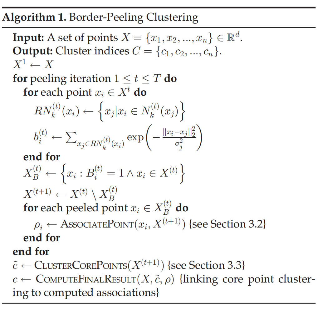
​ The iterative peeling terminates when the identified border points are strictly weaker in terms of their “borderness” than the border points that were identified in the previous iterations, thus forming the set of core points. These core points are then grouped into clusters using a simplified version of DBSCAN. In Algorithm 1, we describe our algorithm in pseudo-code.

当所识别的边界点在“边界性”方面严格弱于在先前迭代中识别的边界点时，迭代剥离终止，从而形成核心点集。然后使用DBSCAN的简化版本将这些核心点分组到集群中。在算法1中，我们用伪代码描述了我们的算法。

​ In what follows, we first introduce some notations and describe how border points are identified at each iteration (Section 3.1). We then detail the border point association process (Section 3.2). Finally, we describe our clustering procedure (Section 3.3).

接下来，我们首先介绍一些符号，并描述如何在每次迭代中识别边界点（第3.1节）。然后我们详细介绍边界点关联过程（第3.2节）。最后，我们描述了我们的聚类过程（第3.3节）。

3.1 Border Points Identification

3.1边界点识别

Given a set of n data points $X= {x_1,x_2,…,x_n} $in ${\mathbb{R}}^d$ and a dissimilarity function $\xi :{\mathbb{R}}^d\times {\mathbb{R}}^d\to \mathbb{R}$ as input, we denote $X^{(t)}$ as the set of points which remain unpeeled by the start of the $t^{th}$ iteration.

给定一组n数据点 $X= {x_1,x_2,…,x_n} $和相异函数$\xi:\mathbb{R^d \times R^d \rightarrow R }$ 作为输入，我们将$X^{（t）}$表示为在$t^{th}$迭代开始时保持未剥离的点集。

​ For each point $x_i\in X^{(t)}$ , denote the set of $k$ nearest neighbor by $N_k^{(t)}(x_i)$. Following [19] and [17], the reverse k nearest neighbors of $x_i$ is given by

对于$X^{(t)}$中的每个点$x_i$，用 $N_k^{(t)}(x_i)$表示最近的邻居$k$的集合。 在[19]和[17]之后，$x_i$的反向k最近邻居由下式给出：
R N k ( t ) ( x i ) = { x j ∣ x i ∈ N k ( t ) ( x j ) } (1) RN^{(t)}_k(x_i)=\{ x_j|x_i\in N_k^{(t)}(x_j) \tag{1} \} RNk(t)​(xi​)={ xj​∣xi​∈Nk(t)​(xj​)}(1)
That is, $R{N}_k^{(t)}(x_i)$is the set of points for which $x_i$ is one of their k-nearest neighbors.

也就是说， $R{N}_k^{(t)}(x_i)$是$x_i$是其k个最近邻居之一的点集。

​ To estimate distances between points, we use a pairwise relationship function f ：${\mathbb{R}}^d\times {\mathbb{R}}^d\to \mathbb{R}$ . In our work, where the dissimilarity measure $\xi$ is the euclidean distance, we calculate f by applying a Gaussian kernel with local scaling [20] to the euclidean distance:
$$f\left(x_i,x_j\right)=\exp \left(-\frac{{\Vert x_i-x_j\Vert }_2^2}{{\sigma }_j^2}\right),\text{\hspace{1em}(2)}$$
Following the choice of ${\sigma }_j$ in [20] we set ${\sigma }_j={\Vert x_j-N_k^{(t)}\left(x_j\right)[k]\Vert }_2$.where N denotes the kth nearest neighbor of $x_j$ at iteration t, i.e., the distance to the $k^{th}$ neighbor of the data point is used as the normalizing factor for the Gaussian kernel. This approach has proven to be effective in measuring the affinity between data points when the affinity of the data points has a large variance.

为了估计点之间的距离，我们使用成对关系函数f：${\mathbb{R}}^d\times {\mathbb{R}}^d\to \mathbb{R}$。 在我们的工作中，相异性度量$ \xi $是欧几里德距离，我们通过对欧几里德距离应用局部缩放[20]的高斯核来计算f：
$$f\left(x_i,x_j\right)=\exp \left(-\frac{{\Vert x_i-x_j\Vert }_2^2}{{\sigma }_j^2}\right),\text{\hspace{1em}(2)}$$
在[20]中选择${\sigma }_j$之后，我们设置${\sigma }_j={\Vert x_j-N_k^{(t)}\left(x_j\right)[k]\Vert }_2$其中N表示迭代t时xj的第k个最近邻居，即，到数据点第k个邻居的距离用作高斯核的归一化因子。 当数据点的亲和力具有大的方差时，这种方法已被证明在测量数据点之间的亲和力方面是有效的。

Using $f$, we associate with each point in $X^{(t)}$ a density influence value $b_i^{(t)}$ where
$$b_i^{(t)}=\sum _{x_j\in R{N}_k^{(t)}\left(x_i\right)}f\left(x_i,x_j\right)\text{\hspace{1em}(3)}$$
The density influence $b_i$ aims at capturing the amount of influence a point has on the local density of its neighboring points. We would expect the values of $b_i$ to be smaller for data points that lie on the border of the cluster, and larger for points that are closer to the core of the cluster. In the supplementary material, which can be found on the Computer Society Digital Library at here. we analytically demonstrate $b_i$’s desired behavior for the simple case where the points are uniformly distributed over a section in ${\mathbb{R}}^1$.

使用$ f $，我们将$ X ^ {（t）} $中的每个点与密度影响值$ b_i ^ {（t）} $关联起来，其中
$$b_i^{(t)}=\sum _{x_j\in R{N}_k^{(t)}\left(x_i\right)}f\left(x_i,x_j\right)\text{\hspace{1em}(3)}$$
密度影响$b_i$的目的是捕获一个点对其相邻点的局部密度的影响程度。 我们希望位于群集边界上的数据点的$b_i$值较小，而靠近群集核心的点的$b_i$值较大。 在补充材料中，可以在此处。我们分析性地证明了$b_i$在点${\mathbb{R}}^1$中的某个部分上均匀分布的简单情况下的理想行为。

Recall that in every peeling iteration, the algorithm classifies some of the points of as border points and peels them off. Formally, for each point $x_i\in X^{(t)}$ , denote by $B_i^{(t)}$ the border classification value of that point that accepts the value of 1 if $x_i$ is a border point and 0 otherwise. The calculation of $B_i^{(t)}$ in each iteration is performed using an iteration specific cut-off value ${\tau }^{(t)}$:
$$B_i^{(t)}=\{\begin{array}{ll}1,& \text{ if }{b}_i^{(t)}\le {\tau }^{(t)}\\ 0,& \text{ otherwise }\end{array}\text{\hspace{1em}(4)}$$
It is important to note that $B_i^{(t)}$ is space-variant due to its reliance on f (through $b_i^{(t)}$). Simply put, we learn the local characteristics of the dataset to determine whether a point is classified as a border point or not. The set of cut-off values can be manually specified, or as we describe below, it can be estimated from the intrinsic properties of the input data.

回想一下，在每个剥离迭代中，该算法将的一些点分类为边界点并将其剥离。 正式地，对于每个点 $x_i\in X^{(t)}$，用 $B_i^{(t)}$ 表示该点的边界分类值，如果$x_i$是边界点，则该边界分类值接受值1 否则为0。 每次迭代中的$B_i^{(t)}$的计算是使用迭代特定的截止值${\tau }^{(t)}$进行的：
$$B_i^{(t)}=\{\begin{array}{ll}1,& \text{ if }{b}_i^{(t)}\le {\tau }^{(t)}\\ 0,& \text{ otherwise }\end{array}\text{\hspace{1em}(4)}$$
重要的是要注意$B_i^{（t）}$是空间可变的，因为它依赖于f（through $b_i^{(t)}$）。 简而言之，我们学习数据集的局部特征，以确定一个点是否被分类为边界点。 截止值集可以手动指定，或者如我们下面所述，可以根据输入数据的固有属性进行估算。

To conclude the peeling iteration, the set of border points at iteration $t$ is given by

为了结束剥离迭代，迭代$ t $的边界点集由下式给出：
$$X_B^{(t)}=\left\{x_i\in X^{(t)}:B_i^{(t)}=1\right\}$$
and the set of unpeeled data points for the next iteration by

以及下一次迭代的未剥离数据点集
$$X^{(t+1)}=X^{(t)}\setminus X_B^{(t)}$$

3.2 Border Points Association

Following the identification of border points at iteration t, we associate to each identified border point $x_i\in X_B(t)$ a neighboring non-border point which we denote as ${\rho }_i\in X^{(t+1)}$. In order to prevent a scenario in which an isolated border point is associated with a relatively distant neighbor, resulting with erroneous merging of distant clusters, we mark some points as outliers. These points will not be part of any cluster.

在迭代t识别出边界点之后，我们将每个标识出的边界点 $x_i\in X_B(t)$与一个相邻的非边界点相关联，记作 ${\rho }_i\in X^{(t+1)}$。 为了防止孤立的边界点与相对较远的邻居相关联而导致对远方群集的错误合并而导致的情况，我们将一些点标记为离群值。 这些点将不属于任何群集。

${\rho }_i$ is given by
$${\rho }_i=\{\begin{array}{ll}{x}_j,& \xi \left(x_i,x_j\right)\le l_i\\ \varnothing ,& \xi \left(x_i,x_j\right)>l_i\end{array}$$
where $x_j$ is the closest non-border point to $x_i$ at iteration $t$ from the set of non-border points and $l_i$ is a spatially-variant threshold value. $\varnothing$ is used to mark $x_i$ as an outlier. In words, if there are no non-border points within a distance of $l_i$ from $x_i$ then $x_i$ is marked as an outlier. Otherwise, ${\rho }_i$ is the nearest non-border point to $x_i$ at iteration $t$.

其中，$x_j$是从非边界点集合中迭代$t$到$x_i$的最接近非边界点，而$l_i$是空间变化的阈值。 $emptyset$用于将$x_i$标记为离群值。 换句话说，如果在$l_i$到$x_i$的距离内没有非边界点，则将$x_i$标记为离群值。 否则，${\rho }_i$是迭代$t$到$x_i$的最近非边界点。

For each border point $x_i$, $l_i$ is determined at the time the point is classified as a border point. All border points identified in the first iteration receive the value of $\lambda$, where $\lambda$ is a parameter of our method which serves as the maximal threshold value. For the subsequent iterations, consider a point $x_i$ at the iteration $t$ where it was peeled. We take the k-nearest data points to $x_i$ from the data points that are in ${\cup }_{r=1}^t{X}_B(r)$, i.e., the set of points that were already peeled up to the current iteration and were not marked as outliers.We denote this set by $N{N}_{b,k}^{(t)}(x_j)$. We then compute

对于每个边界点$x_i$，在将该点分类为边界点时确定$l_i$。第一次迭代中标识的所有边界点均接收$\lambda$的值，其中$\lambda$是我们方法的参数，用作最大阈值。 对于后续迭代，请考虑在迭代$t$处将其剥皮的点$x_i$。 我们将${\cup }_{r=1}^t{X}_B（r)$中的数据点中的k个最近数据点取到$x_i$，即已经剥离的点集直到当前迭代为止，并且未标记为离群值。我们用$N{N}_{b,k}^{(t)}(x_j)$.表示此集合。 然后我们计算
$$l_i=\min \left\{\frac{C}{k}\sum _{x_j\in N{N}_{B,k}^{(t)}}\xi \left(x_i,x_j\right),\lambda \right\}$$
where the constant C determines the strictness of the threshold values (C = 3 in all our experiments).

其中常数C决定阈值的严格性（在我们所有的实验中C = 3）。

We have found this method to perform better than when using a constant threshold value, as it takes into account the spatially-varying density of the data points. See Fig. 2.

我们发现此方法比使用恒定阈值时性能更好，因为它考虑了数据点的空间变化密度。 参见图2。

​

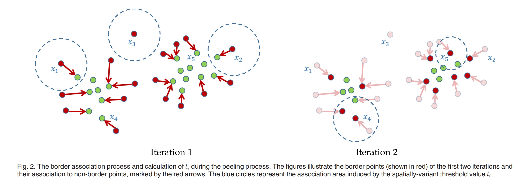
​ Fig. 2 illustrates the effects of the spatially-variant threshold value $l_i$. As the figure demonstrates, at first the association areas (illustrated by blue circles), whose radius equals $l_i$, are of equal size. Some data points (such as $x_3$ in the figure) are not associated to a non-border point since there are no non-border points with distance of at most $\lambda$ . The right figure illustrates the threshold values after one iteration. The values of the newly identified border points are calculated by averaging over the euclidean distances to the nearest peeled border points. Note, for example, that $l_4$ is larger than $l_5$, as $x_4$is further away from its nearest peeled border points (assuming, for instance, k = 3).

图2说明了空间变量阈值$l_i$的影响。如图所示，首先，半径为$l_i$的关联区域(用蓝色圆圈表示)大小相等。有些数据点(如图中的$x_3$)不与非边界点相关联，因为没有距离最多为$\lambda$ 的非边界点。右图说明了一次迭代后的阈值。新识别的边界点的值是通过平均到最近去皮边界点的欧氏距离来计算的。注意，例如，$l_4$大于$l_5$，因为$ x_4 $距离最近的去皮边界点更远(例如，假设k = 3)。

3.3 Bottom-Up Clustering

Our method iteratively identifies border points and associates them to non-border points. The transitive association thus yields paths from each input point to one of the core points, which are the final remaining non-border points, i.e., the set $X^{(T+1)}$with the set that contains ${\rho }_i$. We define a heuristic to set the number of iterations T in a context-sensitive manner (more details are provided in Section 4).

我们的方法迭代地识别边界点并将它们与非边界点关联起来。传递关联因此产生了从每个输入点到一个核心点的路径，这些核心点是最后剩余的非边界点，即集合$X^{(T+1)}$和包含${\rho }_i$的集合。我们定义一个启发式，以上下文敏感的方式设置迭代次数T(更多细节在第4节中提供)。

Once the border peeling process terminates, the remaining set of core points are clustered by merging together close reachable neighborhoods of points. Formally, we define reachable neighborhoods of core points as follows:

一旦边界剥离过程结束，剩余的核心点集通过合并近可达的点邻域聚集在一起。我们正式定义核心点的可达邻域如下:

Definition 3.1. A pair of core points $x_i,x_j \in X^{(T+1)} $is said to be reachable w.l.o.g. if there is a series of core points: $(x_{k_1},...x_{k_m})$with $k_i=i$ and $k_m=j$, such that for every two adjacent indices in the series $(k_r,k_{r+1}$ the relation $\xi \left(x_{k_r},x_{k_{r+1}}\right)\le \max \left(l_{k_r}^{(T)},l_{k_{r+1}}^{(T)}\right)$ holds.

定义3.1。$X^{(T+1)}$中的一对核心点$x_i,x_j$ w.l.o.g是可以到达的。 如果存在一系列核心点：$（x_{k_1},...x_{k_m}）$，其中$k_i=i$和$k_m=j$，则对于该系列中的每两个相邻索引$(k_r，k_{r+1})$关系$\xi \left(x_{k_r},x_{k_{r+1}}\right)\le \max \left(l_{k_r}^{(T)},l_{k_{r+1}}^{(T)}\right)$成立

For every pair of core points $(x_i,x_j)$ that are reachable, we merge the set that contains $x_i$ with the set that contains $x_j$. This merging step is done iteratively, until all sets of reachable data points are merged.

每对核心点 $(x_i,x_j)$，我们合并包含$x_i$的集合和包含$x_j$的集合。这个合并步骤是迭代完成的，直到所有可到达的数据点集合被合并。

The set of cluster candidates are then defined by following the border points association and linkage to the core points. In order to be able and better filter out noise, we mark small clusters as noise, using a user defined value of the minimum cluster size. Following the filtering step, the final set of clusters is returned.

然后通过边界点与核心点的关联和链接来定义集群候选集。为了能够更好地滤除噪声，我们使用用户定义的最小簇大小值将小簇标记为噪声。在过滤步骤之后，返回最后一组集群。

4 EXPERIMENTS

To evaluate the performance of the Border-Peeling clustering method, we measured its performance on numerous synthetic and real-life datasets and compared its performance to other state-of-the-art algorithms. For each experiment, the free parameters of all the alternative methods were set according to their best performance over a large range of possible configurations. Contrarily, for our method, a fixed set of parameters was used throughout all of the experiments. This gives a huge advantage to the alternative methods and demonstrates that our method is insensitive to its parameters setting (which we further validate in a sensitivity evaluation which can be found in the supplementary material, available online).

为了评估边界剥离聚类方法的性能，我们在大量的合成数据集和真实数据集上测试了它的性能，并将它与其他最先进的算法进行了比较。对于每个实验，所有替代方法的自由参数都是根据它们在大范围的可能配置下的最佳性能来设置的。相反，对于我们的方法，在所有的实验中使用一组固定的参数。这为替代方法提供了巨大的优势，并证明了我们的方法对其参数设置不敏感（我们在敏感性评估中进一步验证了这一点，可在补充材料中找到，在线提供）。

​ The free parameters of our method were set as follows: In each iteration,${\tau }^{(t)}$was set such that 90 percent of the remaining data points at each iteration have larger values of $b_i^{(t)}$ , and a value of $k=20$ was used for the k-NN queries. The value of was calculated by first calculating all of the pairwise distances in the k-neighborhood of each point: D k = ⋃ x i ∈ X { d ( x i , x j ) ∣ x j ∈ N k ( x i ) } D_k=\bigcup_{x_i\in X}\{ d(x_i,x_j)|x_j\in N_k(x_i)\} Dk​=⋃xi​∈X​{ d(xi​,xj​)∣xj​∈Nk​(xi​)}and then setting$\lambda =MEAN(D_k)+STD(D_k)$. While other choices of $\lambda$ can be used, we have found this simple estimation method tobe effective, as can be seen in the results below.

我们的方法的自由参数设置如下：在每个迭代中，${\tau }^{（t）}$被设置为每个迭代中90%的剩余数据点具有更大的值$b_i^{(t)}$，k-NN查询使用$k=20$。通过首先计算每个点的k邻域中的所有成对距离来计算的值: D k = ⋃ x i ∈ X { d ( x i , x j ) ∣ x j ∈ N k ( x i ) } D_k=\bigcup_{x_i\in X}\{ d(x_i,x_j)|x_j\in N_k(x_i)\} Dk​=⋃xi​∈X​{ d(xi​,xj​)∣xj​∈Nk​(xi​)}然后设置$\lambda =MEAN(D_k)+STD(D_k)$。虽然可以使用$\lambda$的其他选项，但我们发现这种简单的估计方法是有效的，如后文的结果所示。

​ To automatically set the number of iterations of the peeling process T, we make the following observation: peeled border points should reside in denser areas than the border points of the previous iteration. Therefore, the assigned density influence values should increase in average (which implies that the points establish less coherent borders than the previous iterations). Furthermore, when over-clustering occurs, the values of the border points are expected to be significantly higher than the values of the border points in the preceding iterations.

为了自动设置剥离过程的迭代次数T，我们进行了以下观察：剥离的边界点应该位于比上一次迭代的边界点更密集的区域中。因此，指定的“密度流入”值应平均增加（这意味着这些点建立的边界不如以前的迭代一致）。此外，当发生过度聚类时，期望边界点的值显著高于先前迭代中的边界点的值。

Hence, in each iteration t, we track the set of values of borderpoints that are about to be peeled: { b i ( t ) ∣ B i ( t ) = 1 } \{b_i(t)|B_i^{(t)}=1\} { bi​(t)∣Bi(t)​=1}, and calculate the mean value of that set, denoted by ${\overline{b}}_p^{(t)}$. We then examine the the values of ${\overline{b}}_p^{(1)},{\overline{b}}_p^{(2)},...,{\overline{b}}_p^{(t)}$ and terminate the peeling when $\frac{{\overline{b}}_p^{(t)}}{{\overline{b}}_p^{(t-1)}}-\frac{{\overline{b}}_p^{(t-1)}}{{\overline{b}}_p^{(t-2)}}>ϵ$, where $ϵ$ is a positive constant that we empirically set to 0.15.

因此，在每次迭代*t 中，我们跟踪将要剥离的边界点的值集： { b i ( t ) ∣ B i ( t ) = 1 } \{b_i(t)|B_i^{(t)}=1\} { bi​(t)∣Bi(t)​=1}，并计算平均值 该集合中的一个，用表${\overline{b}}_p^{(t)}$示。 然后，我们检查的值 ${\overline{b}}_p^{(1)},{\overline{b}}_p^{(2)},...,{\overline{b}}_p^{(t)}$ ，并在，其中 $\frac{{\overline{b}}_p^{(t)}}{{\overline{b}}_p^{(t-1)}}-\frac{{\overline{b}}_p^{(t-1)}}{{\overline{b}}_p^{(t-2)}}>ϵ$ 时终止剥离, $\epsilon $是我们根据经验将其设置为0.15的常数。

We compare our performance to that of a set of well-known non-parametric clustering techniques: DBSCAN (DB) and the more recent Hierarchical-DBSCAN (HDB) [9], Mean-Shift (MS), Affinity Propagation (AP) [16], QCC [18] and Robust Continuous Clustering(RCC) [21]. Similar to Border-Peeling clustering, all of those clustering methods try to infer the number of clusters automatically and do not accept the number of clusters as a parameter. We also compare our performance to the K-Means (KM) and Spectral Clustering (SC) [22] methods, which accept the number of clusters as a parameter. For each dataset, we run K-Means 1000 times with random initialization, taking the clustering which minimizes the sum of distances of data points to their closest cluster center among those 1000 runs. Similarly, for Spectral Clustering, the K-Means phase is also run 1000 times, taking the best result among these runs.

我们将性能与一组著名的非参数聚类技术的性能进行比较：DBSCAN（DB）和最新的Hierarchical-DBSCAN（HDB）[9]，均值漂移（MS），亲和力传播（AP）[ 16]，QCC [18]和鲁棒连续聚类（RCC）[21]。 与边界剥离群集相似，所有这些群集方法都尝试自动推断群集的数量，并且不接受群集的数量作为参数。 我们还将性能与K-Means（KM）和光谱聚类（SC）[22]方法进行比较，后者将聚类数作为参数。 对于每个数据集，我们使用随机初始化对K-Means进行了1000次运行，进行了聚类，这使数据点到这1000次运行中最接近的聚类中心的距离之和最小。 同样，对于光谱聚类，K-Means阶段也运行1000次，在这些运行中获得最佳结果。

In what follows, we explain and demonstrate our quantitative comparisons on three synthetic datasets as well as on sampled large datasets. In the supplementary material, available online, we provide qualitative results on six additional synthetic datasets of various distributions and further illustrate the huge advantage we provide the alternative techniques by presenting the entire grid of results. While all our results are obtained with a fifixed set of parameters, we explicitly demonstrate how for alternative methods a fixed parameter setting will work well for only some of the scenarios.

接下来，我们将解释和演示我们在三个合成数据集以及大型采样数据集上的定量比较。 在在线提供的补充材料中，我们在六个其他各种分布的综合数据集上提供了定性结果，并通过展示整个结果网格进一步说明了我们提供替代技术的巨大优势。 虽然我们所有的结果都是通过一组固定的参数获得的，但是我们明确地演示了对于固定方法，固定参数设置仅在某些情况下如何才能很好地工作。

4.1 Evaluation on Common Synthetic Datasets

First, we quantitatively evaluated our method on a number of common synthetic datasets from the known clustering literature [23], [24], [25], which consist of a small number of clusters that lie in proximity to one another and are not easily separable, thus constituting a challenge to density-based methods. We provide a comparative visualization of the clusters formed by Border-Peeling clustering to the clusters formed by K-Means and Spectral Clustering, to demonstrate that our non-parametric clustering method outperforms parametric techniques even in synthetic settings (see Fig. 3).

首先，我们从已知的聚类文献[23]，[24]，[25]的许多通用合成数据集中对我们的方法进行了定量评估，这些数据集由彼此靠近且不容易的少量聚类组成 可分离性，因此对基于密度的方法构成了挑战。 我们提供了一个由边界剥离聚类形成的聚类与由K均值和光谱聚类形成的聚类的比较可视化结果，以证明即使在合成设置中，我们的非参数聚类方法也优于参数化技术（参见图3）。

We evaluate the performance of each method by calculating the Adjusted Rand Index (ARI) [26] and Adjusted Mutual Information (AMI) [27] of the resulting metrics. The ARI and AMI are well known metrics in the field of data clustering and are frequently used in order to evaluate clustering performance when ground truth data is available. The scores for the well-known clustering methods were obtained by running them over a range of parameters and taking the clustering result with the best AMI score, while Border-Peeling clustering was run using the parameters described in the previous section. See Table 1 for the full comparison on these synthetic datasets. As Fig. 3 demonstrates, our technique successfully identified the number of clusters for each of the datasets and achieved the best scores overall.

我们通过计算所得指标的调整后的兰德指数（ARI）[26]和调整后的相互信息（AMI）[27]来评估每种方法的性能。 ARI和AMI是数据聚类领域中众所周知的指标，并且在有地面真实数据可用时，经常使用ARI和AMI来评估聚类性能。 众所周知的聚类方法的分数是通过在一系列参数上运行并获得具有最佳AMI分数的聚类结果而获得的，而Border-Peeling聚类是使用上一节中描述的参数来运行的。 有关这些综合数据集的完整比较，请参见表1。 如图3所示，我们的技术成功地识别了每个数据集的聚类数量，并总体上获得了最佳分数。

4.2 Evaluation on Large Datasets

We further evaluated the performance of the Border-Peeling method in comparison to other well-known clustering algorithms by running it on large datasets. We perform two different sets of experiments: (i) experiments on unsupervised features and (ii) experiments on supervised (pretrained) features. As can be expected, the results are generally better on the supervised features. However, as the evaluation illustrates, clustering a large dataset is challenging even in a supervised setting (see Fig. 4 for a visualization of the supervised features). Our evaluation shows that our method is competitive to other state-of-the-art techniques in both cases. It is important to note that throughout our experiments, the Border-Peeling parameters were fixed as described above, while the parameters of the other techniques were set separately for each dataset by taking the parameters that yield the best result. Furthermore, note that in this section, we only partially compare to the QCC technique as their implementation is in MATLAB, making it infeasible to run all the different confifigurations on these large datasets.

通过在大型数据集上运行，我们进一步评估了与其他众所周知的聚类算法相比，Border-Peeling方法的性能。我们执行两组不同的实验：（i）在无监督特征上进行实验，以及（ii）在有监督（预训练）下进行特征的实验。可以预料，在受监督的功能上效果通常会更好。但是，如评估所示，即使在有监督的环境中，对大型数据集进行聚类也具有挑战性（有关受监督特征的可视化，请参见图4）。我们的评估表明，在两种情况下，我们的方法都与其他最新技术竞争。重要的是要注意，在我们的整个实验中，如上所述，Border-Peeling参数是固定的，而其他技术的参数是通过采用产生最佳结果的参数分别为每个数据集设置的。此外，请注意，在本节中，我们仅部分比较了QCC技术，因为它们是在MATLAB中实现的，因此无法在这些大型数据集上运行所有不同的配置。

4.2.1 Experiments on Unsupervised Feature Vectors

We conducted a set of experiments on larger datasets (approximately 10,000 samples) of varying classes, where the feature vectors are generated using auto-encoders. For all the experiments, we used auto encoder dimensions of $dim(X)-500-500-2000-10$ . The training of the autoencoder included 50 epochs of layerwise training, followed by 50 additional epochs for fifine-tuning the entire autoencoder.

我们对不同类别的较大数据集（大约10,000个样本）进行了一组实验，其中使用自动编码器生成了特征向量。 对于所有实验，我们使用的自动编码器尺寸为$ dim（X）-500-500-2000-10 $。 自动编码器的训练包括50个时期的分层训练，然后是50个额外的时期，用于对整个自动编码器进行微调。

In Table 2, we report a full quantitative comparison on the YouTube Faces (YTF) dataset [28] which contains 10,000 samples of faces, on the USPS dataset which contains 11,000 samples of handwritten digits, and on the REUTERS dataset which contains 10,000 samples of English news stories [29]. As the table illustrates, our method obtains competitive performance on all three datasets, also in comparison to parametric methods that are provided with the number of clusters in the data. Furthermore, our method does not over-segment these large datasets (unlike some of the other methods). In the supplementary material, available online, we demonstrate that our method is insensitive to small variations of its automatically estimated parameter by reporting our scores on these datasets over a wide range of different parameter values.

在表2中，我们报告了YouTube面孔（YTF）数据集[28]（其中包含10,000个面孔样本），USPS数据集（包含11,000个手写数字样本）以及REUTERS数据集（其中包含10,000个面孔样本）进行了全面的定量比较。 英语新闻故事[29]。 如表所示，我们的方法在所有三个数据集上均具有竞争优势，与数据中聚类数量提供的参数方法相比也是如此。 此外，我们的方法不会过度分割这些大型数据集（与其他一些方法不同）。 在在线提供的补充材料中，我们通过报告这些数据集在各种不同参数值范围内的得分，证明了该方法对其自动估算参数的细微变化不敏感。

4.2.2 Experiments on Supervised Feature Vectors

To further validate the performance of our technique on large datasets, we generated large sets by extracting feature vectors generated by convolutional neural networks (CNN) that were trained separately on MNIST [30]. MNIST is a well-known handwritten digit image dataset which consists of 70000 labeled images of handwritten digits divided into a training set of 60,000 images and a test set of 10,000 images.

为了进一步验证我们的技术在大型数据集上的性能，我们通过提取由卷积神经网络（CNN）生成的特征向量来生成大型集合，这些特征向量在MNIST上进行了单独训练[30]。 MNIST是一个著名的手写数字图像数据集，由70000个带标签的手写数字图像组成，分为60,000张图像的训练集和10,000张图像的测试集。

To obtain a strong feature representation on the MNIST samples, we trained a CNN using the training set and then used it to produce an embedding of the images in the test set to n-dimensional feature vectors (n=500). To obtain the feature vectors, we used the CNN implementation which is available in the MatConvNet [31] library. To produce varying less balanced datasets with an unknown number of clusters, the embedded test sets were sampled by taking all the embedded vectors which are within a certain radius of randomly sampled points. By using different radii, we generated several datasets of varying sizes. The selected radii values yielded varying datasets containing roughly a few thousand elements, spanning most, but not necessarily all, the digits (as illustrated on the top of Table 3). On average, the number of sampled images is 2151, 3115, 4321 and 4471 for radius size 120, 130, 140 and 150, respectively. Embeddings of selected samples of the MNIST dataset to 2D can be seen in Fig. 4. As a final preprocessing step, we employed PCA on the sampled datasets to avoid clustering in an overly-high dimensional space, reducing the original dimensions down to 30.

为了在MNIST样本上获得强大的特征表示，我们使用训练集对CNN进行了训练，然后将其用于将测试集中的图像嵌入到n维特征向量（n = 500）中。为了获得特征向量，我们使用了MatConvNet [31]库中可用的CNN实现。为了产生具有未知数目簇的变化不平衡的数据集，通过取在随机采样点的一定半径内的所有嵌入矢量来对嵌入测试集进行采样。通过使用不同的半径，我们生成了多个大小不同的数据集。选定的半径值产生了包含大约数千个元素的变化的数据集，这些元素跨越了大多数（但不一定是全部）数字（如表3顶部所示）。平均而言，半径大小为120、130、140和150的采样图像数分别为2151、3115、4321和4471。 MNIST数据集的选定样本到2D的嵌入可以在图4中看到。作为最后的预处理步骤，我们在样本数据集上采用了PCA，以避免在过高的维空间中聚类，从而将原始维减少到30。

The results of running Border-Peeling clustering as well as the other non-parametric clustering techniques are illustrated in Table 3. For each radii value, we perform ten different runs and average the results of the clustering methods over these random runs. As a baseline, we also report the results on the full (not- sampled) datasets.

表3说明了运行Border-Peeling聚类以及其他非参数聚类技术的结果。对于每个半径值，我们执行十次不同的运行，并对这些随机运行的聚类方法的结果求平均。 作为基准，我们还报告了完整（未采样）数据集的结果。

As the table demonstrates, RCC and our technique achieve the best performance on average in terms of AMI and ARI, and for larger radii values our method outperforms the RCC technique. It is especially interesting to observe the huge variability in performance in this experiment where the features are obtained in a supervised fashion and indeed, for some methods, the scores are rather high in most cases. However, it seems that some common clustering solutions do not scale up to the large dataset size or the high dimensional feature space of the real image samples, even when provided with the supervised feature vectors. Furthermore, these experiments also demonstrate that our proposed method avoids over-partitioning to some degree, in particular in comparison to other methods.

如表所示，RCC和我们的技术在AMI和ARI方面平均取得最佳性能，对于较大的半径值，我们的方法优于RCC技术。 特别有趣的是，在此实验中观察到性能的巨大差异，其中以监督方式获得特征，实际上，对于某些方法，大多数情况下得分都很高。 但是，即使提供了监督的特征向量，似乎某些常见的聚类解决方案也无法扩展到实际图像样本的大数据集大小或高维特征空间。 此外，这些实验还证明，我们提出的方法在某种程度上避免了过度分割，特别是与其他方法相比。

Our incremental peeling process can also infer a confidence value associated with the data points of each cluster. As discussed in Section 3.1, data points with lower values of bi are expected to be along the border of the cluster, and thus, with a lower confidence. To illustrate this simple confifidence ranking, Fig. 5 visualizes the top-10 and bottom-10 instances of clustering the MNIST dataset. Note that the images of digits with lower values of $b_i^{(0)}$ are often harder to identify, while images with higher values are clearer and more pronounced.

我们的增量剥离过程还可以推断与每个群集的数据点相关的置信度值。 如第3.1节所述，具有较低bi值的数据点预计将沿着群集的边界，因此具有较低的置信度。 为了说明这种简单的置信度排名，图5可视化了MNIST数据集聚类的前10个和后10个实例。 请注意， $b_i^{(0)}$值较低的数字图像通常较难识别，而值较高的图像则更清晰，更清晰。

4.3 Implementation Details and Runtime

The Border-Peeling clustering method was implemented in the Python programming language using the numpy [32] software library. In order to compare our performance with other clustering algorithms we used the implementation available in the SciKit-Learn [33] Python library. The time complexity of our technique is $O\left(T\cdot \left(k\cdot n+{\tilde{f}}_{knn}\right)\right)$, where ${\tilde{f}}_{knn}$ is the asymptotic complexity of the method with respect to the dataset.

使用numpy [32]软件库以Python编程语言实现了Border-Peeling聚类方法。 为了将我们的性能与其他聚类算法进行比较，我们使用了SciKit-Learn [33] Python库中提供的实现。 我们的技术的时间复杂度是$O\left(T\cdot \left(k\cdot n+{\tilde{f}}_{knn}\right)\right)$，其中是 ${\tilde{f}}_{knn}$方法相对于数据集的渐近复杂度。

The runtime performance on a 2.5 GHz Intel Core i7 Mac-Book Pro on the datasets evaluated in Section 4.2.1 is as follows: 71 seconds on the YTF dataset (T = 19), 98 seconds on the USPS dataset (T = 36), and 106 seconds on the REUTERS dataset (T = 23). For comparison, the average runtime of a single run of the RCC technique on these datasets is 36 seconds, 65 seconds, and 55 seconds, respectively. The implementation of our method is available at: https://github.com/nadavbar/BorderPeelingClustering.

在第4.2.1节中评估的数据集上，在2.5 GHz Intel Core i7 Mac-Book Pro上的运行时性能如下：YTF数据集（T = 19）上为71秒，USPS数据集（T = 36）上为98秒 ，以及REUTERS数据集上的106秒（T = 23）。 为了进行比较，在这些数据集上一次运行RCC技术的平均运行时间分别为36秒，65秒和55秒。 我们的方法的实现可在以下网址获得：https：//github.com/nadavbar/BorderPeelingClustering。

5 CONCLUSIONS

We have presented a non-parametric clustering technique that groups points into different clusters by iteratively identifying points that reside on the borders of the cluster and removing them until separable areas of data remain. During the peeling process, the method creates associations between the peeled border points and points in the inner layers by estimating the local density of the data points. These associations are then used to link between the separable unpeeled data points and thus form the resulting clusters.

我们提出了一种非参数聚类技术，该技术通过迭代识别位于聚类边界上的点并将其移除，直到数据的可分离区域保留下来，从而将点分组到不同的聚类中。在剥离过程中，该方法通过估计数据点的局部密度，在剥离的边界点和内层点之间建立关联。然后，这些关联被用于在可分离的无eeled数据点之间进行链接，从而形成结果簇。

​ The main idea of the method is the peeling of the border points which ensures that the cores of near-by clusters are clearly separated before the data points are classified as separate clusters. We present a novel formulation for identifying border points, which we validated analytically on a simple setting of a uniformly-distributed cluster. Additionally, as we have shown above, our border peeling technique can be used to infer confidence values associated with the data points of each cluster. Unlike other methods, we do not make strong assumptions about the structure of the data points or their density distribution such as a single density peak or uniform density levels. Our approach can cope with multiple distribution models, as kNN neighborhoods, unlike -neighborhoods, are not affected by varying distributions in the data. Furthermore, the method has been shown to be stable in the sense that it is insensitive to the setting of hard coded parameters.

该方法的主要思想是边界点的剥离，在数据点被划分为独立的簇之前，保证了相邻簇的核心被清晰地分离。我们提出了一种新的边界点识别公式，并在一个简单的均匀分布簇上进行了分析验证。此外，正如我们上面所示，我们的边界剥离技术可以用来推断与每个簇的数据点相关联的置信值。与其他方法不同，我们不对数据点的结构或其密度分布（如单个密度峰值或均匀密度水平）作出强有力的假设。我们的方法可以处理多种分布模型，因为kNN邻域不同于-邻域，不受数据中不同分布的影响。此外，该方法对硬编码参数的设置不敏感，因此是稳定的。

​ We have extensively analyzed the performance of the Border-Peeling method over large datasets for which the number of clusters is unknown, and there is no prior knowledge about its general structure or density distribution. As we have shown, Border-Peeling clustering is competitive to other state-of-the-art non-parametric clustering methods, even when their free parameters are fine-tuned to achieve their best performance. In particular, the performance of Border-Peeling in comparison to DBSCAN is interesting since conceptually the two techniques have much in common, as both methods extract the core of the clusters that separate adjacent clusters, and then expand core points to the rest of the cluster. However, the difference in performance is intriguing. We attribute the better performance of Border-Peeling clustering to the fact that the core points are not defined globally, but through an iterative process that senses the local densities. The incremental peeling not only identifies the border points but also carefully associates them with points that seem to be closer to the core of the cluster. Furthermore, the locally adaptive approach is advantageous in sensing and avoiding over-segmentation of the clusters. Having said that, we believe that the more significant advantage of Border-Peeling over DBSCAN and other non-parametric clustering methods is that the method is insensitive to small variations in parameter values, and that those values can be easily set according to the characteristics of the data set, as can be seen in the experiments section.

我们广泛地分析了边界剥离方法在大数据集上的性能，对于这些数据集，簇的数目是未知的，并且没有关于其一般结构或密度分布的先验知识。如我们所示，边界剥离聚类与其他最先进的非参数聚类方法相比具有竞争力，即使对其自由参数进行微调以获得最佳性能。特别是，与DBSCAN相比，边界剥离的性能是有趣的，因为这两种技术在概念上有很多共同点，因为这两种方法都提取分隔相邻簇的簇的核心，然后将核心点扩展到簇的其余部分。然而，在性能上的差异是耐人寻味的。我们将边界剥离聚类的更好性能归因于核心点不是全局定义的，而是通过一个感知局部密度的迭代过程。增量剥离不仅可以识别边界点，还可以仔细地将它们与看起来更接近集群核心的点相关联。此外，局部自适应方法有利于检测和避免聚类的过度分割。尽管如此，我们相信边界剥离比DBSCAN和其他非参数聚类方法更显著的优点是，该方法对参数值的微小变化不敏感，并且可以根据数据集的特征轻松地设置这些值，如实验部分所示。

All our results were generated with the same set of parameters, which is detailed in the paper. To control the maximum association distance between data points, we estimated (introduced in Section 3.2) according to the global behavior of the data. We believe that this global estimation can be further refifined to better suit datasets with different structures and densities, perhaps in a semi-supervised setting where some samples are labeled. In general, as future work, we believe that our unsupervised technique can be expanded to accommodate supervised scenarios, to achieve improved accuracy in such controlled settings.

我们所有的结果都是用相同的参数集生成的，这在本文中有详细的描述。为了控制数据点之间的最大关联距离，我们根据数据的全局行为来估计（在第3.2节中介绍）。我们相信，这种全局估计可以进一步重新定义，以便更好地适应具有不同结构和密度的数据集，也许是在半监督环境中，其中一些样本被标记。总的来说，作为未来的工作，我们相信我们的无监督技术可以扩展到适应有监督的场景，以提高在这种受控环境中的准确性。

REFERENCES

[1] J. MacQueen, et al., “Some methods for classifification and analysis of multivariate observations,” in Proc. 5th Berkeley Symp. Math. Statist. Probability,1967, pp. 281–297.

[2] Y. Cheng, “Mean shift, mode seeking, and clustering,” IEEE Trans. Pattern Anal. Mach. Intell., vol. 17, no. 8, pp. 790–799, Aug. 1995.

[3] M. Ester, H.-P. Kriegel, J. Sander, and X. Xu, “A density-based algorithm for discovering clusters in large spatial databases with noise.” in Proc. 2nd Int. Conf. Knowl. Discovery Data Mining, 1996, vol. 96, no. 34, pp. 226–231.

[4] A. K. Jain, “Data clustering: 50 years beyond k-means,” Pattern Recognit. Lett., vol. 31, no. 8, pp. 651–666, 2010.

[5] G. Karypis, E.-H. Han, and V. Kumar, “Chameleon: Hierarchical clustering using dynamic modeling,” IEEE Comput., vol. 32, no. 8, pp. 68–75, Aug. 1999.

[6] A. Karami and R. Johansson, “Choosing dbscan parameters automatically using differential evolution,” Int. J. Comput. Appl., vol. 91, no. 7, pp. 1–11, 2014.

[7] K. Sawant, “Adaptive methods for determining dbscan parameters,” Int. J. Innovative Sci. Eng. Technol., vol. 1, no. 4, pp. 329–334, 2014.

[8] M. Ankerst, M. M. Breunig, H.-P. Kriegel, and J. Sander, “Optics: Ordering points to identify the clustering structure,” ACM Sigmod Record, vol. 28, no. 2, pp. 49–60, 1999.

[9] R. J. Campello, D. Moulavi, and J. Sander, “Density-based clustering based on hierarchical density estimates,” in Advances in Knowledge Discovery and Data Mining. New York, NY, USA: Springer, 2013.

[10] L. Ert€oz, M. Steinbach, and V. Kumar, “Finding clusters of different sizes, shapes, and densities in noisy, high dimensional data,” in Proc. 3rd SIAM Int. Conf. Data Min., 2003, pp. 47–58.

[11] D. Cheng, Q. Zhu, and Q. Wu, “A local cores-based hierarchical clustering algorithm for data sets with complex structures,” in Proc. IEEE 42nd Annu. Comput. Softw. Appl. Conf., 2018, vol. 1, pp. 410–419.

[12] D. Cheng, Q. Zhu, J. Huang, Q. Wu, and L. Yang, “A hierarchical clustering algorithm based on noise removal,” Int. J. Mach. Learn. Cybern., vol. 10, pp. 1–12, 2018.

[13] M. Maier, M. Hein, and U. Von Luxburg, “Cluster identifification in nearestneighbor graphs,” in Proc. Int. Conf. Algorithmic Learn. Theory, 2007, pp. 196–210.

[14] I. Shimshoni, B. Georgescu, and P. Meer, “Adaptive mean shift based clustering in high dimensions,” Nearest-Neighbor Methods Learn. Vis.: Theory Practice, pp. 203–220, 2006. [Online]. Available: https://scholar.googleusercontent.com/scholar.bib?q=info:x0NkOLE4kmQJ:scholar.google.com/&output=citation&scisdr=CgW3kWuxEPPMqMTmjI8:AAGBfm0AAAAAXR7jlI_vZmdayujVO9kMI5_WDaqlomqe&scisig=AAGBfm0AAAAAXR7jlGDopngN8bJu0YHAsWMKfICH25Nd&scisf=4&ct=citation&cd=-1&hl=iw

[15] M. A. Carreira-Perpinan, “A review of mean-shift algorithms for clustering,” CRC Handbook of Cluster Anal., pp. 1–28, 2015.

[16] B. J. Frey and D. Dueck, “Clustering by passing messages between data points,” Sci., vol. 315, no. 5814, pp. 972–976, 2007.

[17] C. Xia, W. Hsu, M. L. Lee, and B. C. Ooi, “Border: Effificient computation of boundary points,” IEEE Trans. Knowl. Data Eng., vol. 18, no. 3, pp. 289–303, Mar. 2006.

[18] J. Huang, Q. Zhu, L. Yang, D. Cheng, and Q. Wu, “Qcc: A novel clustering algorithm based on quasi-cluster centers,” Mach. Learn., vol. 106, no. 3, pp. 337–357, 2017.

[19] F. Korn and S. Muthukrishnan, “Inflfluence sets based on reverse nearest neighbor queries,” ACM SIGMOD Record, vol. 29, pp. 201–212, 2000.

[20] L. Zelnik-Manor and P. Perona, “Self-tuning spectral clustering,” in Proc. 17th Int. Conf. Neural Inf. Process. Syst., 2004, pp. 1601–1608.

[21] S. A. Shah and V. Koltun, “Robust continuous clustering,” Proc. Nat. Acad. Sci., vol. 114, no. 37, pp. 9814–9819, 2017.

[22] A. Y. Ng, M. I. Jordan, Y. Weiss, et al., “On spectral clustering: Analysis and an algorithm,” in Proc. 14th Int. Conf. Neural Inf. Process. Syst., 2002, vol. 2, pp. 849–856.

[23] L. Fu and E. Medico, “Flame, a novel fuzzy clustering method for the analysis of dna microarray data,” BMC Bioinformatics, vol. 8, no. 1, p. 3, 2007.

[24] A. Gionis, H. Mannila, and P. Tsaparas, “Clustering aggregation,” ACM Trans. Knowl. Discovery Data, vol. 1, 2007. Art. no. 4.

[25] C. J. Veenman, M. J. Reinders, and E. Backer, “A maximum variance cluster algorithm,” IEEE Trans. Pattern Anal. Mach. Intell., vol. 24, no. 9, pp. 1273–1280, Sep. 2002.

[26] L. Hubert and P. Arabie, “Comparing partitions,” J. Classifification, vol. 2, no. 1, pp. 193–218, 1985.

[27] N. X. Vinh, J. Epps, and J. Bailey, “Information theoretic measures for clusterings comparison: Variants, properties, normalization and correction for chance,” J. Mach. Learn. Res., vol. 11, pp. 2837–2854, 2010.

[28] L. Wolf, T. Hassner, and I. Maoz, “Face recognition in unconstrained videos with matched background similarity,” in Proc. IEEE Conf. Comput. Vis. Pattern Recognit., 2011, pp. 529–534.

[29] D. D. Lewis, Y. Yang, T. G. Rose, and F. Li, “Rcv1: A new benchmark collection for text categorization research,” J. Mach. Learn. Res., vol. 5, no. Apr, pp. 361–397, 2004.

[30] Y. LeCun and C. Cortes, “MNIST handwritten digit database,” 2010. [Online]. Available: http://yann.lecun.com/exdb/mnist/

[31] A. Vedaldi and K. Lenc, “Matconvnet – convolutional neural networks for matlab,” in Proc. ACM Int. Conf. Multimedia, 2015, pp. 689–692.

[32] S. Van Der Walt, S. C. Colbert, and G. Varoquaux, “The numpy array: A structure for effificient numerical computation,” Comput. Sci. Eng., vol. 13, no. 2, pp. 22–30, 2011.

[33] F. Pedregosa, G. Varoquaux, A. Gramfort, V. Michel, B. Thirion, O. Grisel, M. Blondel, P. Prettenhofer, R. Weiss, V. Dubourg, J. Vanderplas, A. Passos, D. Cournapeau, M. Brucher, M. Perrot, and E. Duchesnay, “Scikit-learn: Machine learning in Python,” J. Mach. Learn. Res., vol. 12, pp. 2825–2830, 2011.