在 Wide&Deep 模型 的基础上,改进 Wide 部分,用 Cross network 代替,自动进行特征选择,不像 Wide&Deep 那样需要人工选择特征
Cross Network 每次加入了input 增加一个阶数 参数共享
1 摘要
-
DNN generate all the interactions implicitly, and are not necessarily efficient in learning all types of cross features
DNN 隐式地生成所有的交互,这不一定有效地学习所有类型的交叉特征这里所有类型并不清楚,可能指低阶和高阶特征。文中说 DCN 可以学到某种有限度的特征交互 (certain bounded-degree feature interactions)
-
DCN explicitly applies feature crossing at each layer, requires no manual feature engineering, and adds negligible extra complexity to the DNN model
DCN 明确地在每一层应用特征交叉,不需要人工进行特征工程,并且为 DNN 模型增加了可忽略的额外复杂性这里是要对比 Wide&Deep 的人为选取特征,但其实就是 DNN 的工作
2 介绍
- Identifying frequently predictive features and at the same time exploring unseen or rare cross features is the key to making good predictions
识别频繁的预测特征,同时探索不可见或罕见的交叉特征是做出良好预测的关键这里频繁的预测特征应该指的是像 Wide&Deep 中人为选取的很重要的特征
2.1 相关工作
-
Deep Crossing extends residual networks and achieves automatic feature learning by stacking all types of inputs.
Deep Crossing 扩展了剩余网络,并通过叠加所有类型的输入来实现自动特征学习。 -
DNNs are able to approximate an arbitrary function under certain smoothness assumptions to an arbitrary accuracy, given sufficiently many hidden units or hidden layers 1 2
在给定足够多的隐单元或隐层的情况下,DNN 能够在一定的光滑度假设下,将任意函数近似到任意精度 -
In the Kaggle competition, the manually craſted features in many winning solutions are low-degree, in an explicit format and effective.This has shed light on designing a model that is able to learn bounded-degree feature interactions more efficiently and explicitly than a universal DNN.
在 Kaggle 的比赛中,许多获胜的解决方案中的人工构造特征是低阶的,是明确的格式且有效。这告诉我们要设计一个能够比通用 DNN 更有效、更明确地学习有限度特征交互的模型。Wide&Deep 模型将手动选择的交叉的特征放入线性模型并和一个 DNN 联合训练,本文就想自动地学习特征,而不是手动选择
2.2 主要工作
-
DCN efficiently captures effective feature interactions of bounded degrees, learns highly nonlinear interactions, requires no manual feature engineering or exhaustive searching, and has low computational cost.
DCN 能有效地捕获有效的有限度特征交互,学习高度非线性特征的交互,无需人工特征工程或穷尽搜索,这样计算量小 -
DCN has lower logloss than a DNN with nearly an order of magnitude fewer number of parameters.
DCN 比 DNN 具有更低的 logloss,其参数数目几乎少了一个数量级
3 网络结构
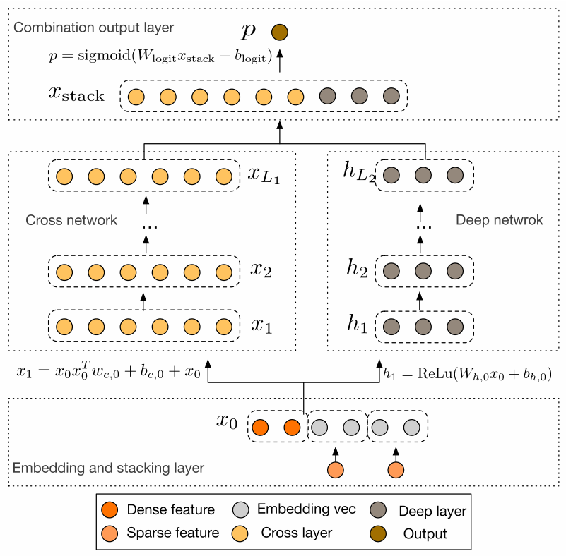
3.1 Embedding and Stacking layer
-
To reduce the dimensionality, we employ an embedding procedure to transform these binary features into dense vectors of real values (commonly called embedding vectors)
为了降低维数,我们采用了一种 Embedding 方法,将这些编码后的类别特征转换为实值的稠密向量(通常称为嵌入向量) -
In the end, we stack the embedding vectors, along with the normalized dense features x d e n s e x_{dense} xdense, into one vector:
最后,把 Embedding 向量和归一化后的稠密向量堆积放入一个向量得
x 0 = [ x embed, 1 T , … , x embed, , k T , x dense T ] (1) \mathbf{x}_{0}=\left[\mathbf{x}_{\text {embed, } 1}^{T}, \ldots, \mathbf{x}_{\text {embed, }, k}^{T}, \mathbf{x}_{\text {dense }}^{T}\right] \tag{1} x0=[xembed, 1T,…,xembed, ,kT,xdense T](1)
3.2 Cross Network
-
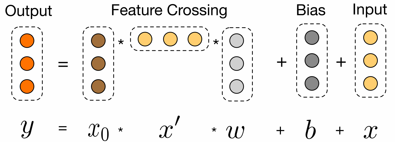
每一个交叉层形式:
x l + 1 = x 0 x l T w l + b l + x l = f ( x l , w l , b l ) + x l (2) \mathbf{x}_{l+1}=\mathbf{x}_{0} \mathbf{x}_{l}^{T} \mathbf{w}_{l}+\mathbf{b}_{l}+\mathbf{x}_{l}=f\left(\mathbf{x}_{l}, \mathbf{w}_{l}, \mathbf{b}_{l}\right)+\mathbf{x}_{l} \tag{2} xl+1=x0xlTwl+bl+xl=f(xl,wl,bl)+xl(2) Each cross layer adds back its input aſter a feature crossing f f f, and the mapping function f : R d ↦ R d f:\mathbb{R}^d \mapsto \mathbb{R}^d f:Rd↦Rd fits the residual of x l + 1 − x l x_{l+1} − x_l xl+1−xl
每个交叉层在特征交叉后再添加输入,函数 f f f 满足 x l + 1 − x l x_{l+1} - x_l xl+1−xl 的残差
-
Let L c L_c Lc denote the number of cross layers, and d denote the input dimension. the number of parameters involved in the cross network is
L c L_c Lc 表示交叉层的数目, d d d 表示输入的维度,cross network 的参数是
d × L c × 2 (3) d \times L_c \times 2 \tag{3} d×Lc×2(3) -
In fact, the cross network comprises all the cross terms x 1 α 1 x 2 α 2 ⋯ x d α d x^{\alpha_1}_1x^{\alpha_2}_2 \cdots x^{\alpha_d}_d x1α1x2α2⋯xdαd of degree from 1 to l + 1 l+1 l+1
事实上,交叉网络包含了所有从 1 到 l + 1 l+1 l+1 阶数的交叉项 -
The time and space complexity of a cross network are linear in input dimension.This efficiency benefits from the rank-one property of x 0 x l T x_0x^T_l x0xlT , which enables us to generate all cross terms without computing or storing the entire matrix.
交叉网络的时间和空间复杂度在输入维度上是线性的,这种效率得益于 x 0 x l T x_0x ^ T_l x0xlT 的秩为1的属性,这使我们能够生成所有交叉项而无需计算或存储整个矩阵
3.3 Combination Layer
- The combination layer concatenates the outputs fromtwo networks and feed the concatenated vector into a standard logits layer.
组合层将两个网络的输出连接起来,并将连接的向量馈送到标准 logits 层
p = σ ( [ x L 1 T , h L 2 T ] w logits ) (4) p=\sigma\left(\left[\mathrm{x}_{L_{1}}^{T}, \mathbf{h}_{L_{2}}^{T}\right] \mathbf{w}_{\text {logits }}\right) \tag{4} p=σ([xL1T,hL2T]wlogits )(4) - The loss function is the log loss alongwith a L 2 L_2 L2 regularization term.
损失函数是 log 损失以及 L 2 L_2 L2 正则化项
loss = − 1 N ∑ i = 1 N y i log ( p i ) + ( 1 − y i ) log ( 1 − p i ) + λ ∑ l ∥ w l ∥ 2 (5) \text { loss }=-\frac{1}{N} \sum_{i=1}^{N} y_{i} \log \left(p_{i}\right)+\left(1-y_{i}\right) \log \left(1-p_{i}\right)+\lambda \sum_{l}\left\|\mathbf{w}_{l}\right\|^{2} \tag{5} loss =−N1i=1∑Nyilog(pi)+(1−yi)log(1−pi)+λl∑∥wl∥2(5)
4 相关工作
-
The cross network shares the spirit of parameter sharing as the FM model and further extends it to a deeper structure.
交叉网络采取了 FM 模型的参数共享想法,并拓展到了更深的结构中 -
Both models have each feature learned some parameters independent from other features, and the weight of a cross term is a certain combination of corresponding parameters
两个模型的每个特征都有一组其他特征无关的参数,并且交叉项的权重是相应参数的某种组合这个交叉网络的想法来自于 FM,把特征交互的阶数延伸
-
Parameter sharing not onlymakes the model more efficient, but also enables the model to generalize to unseen feature interactions and bemore robust to noise
参数共享不仅使模型更有效,而且同时也使模型能够泛化得到看不见的特征交互,并且对噪声更加鲁棒
5 总结
-
The Deep & Cross Network can handle a large set of sparse and dense features, and learns explicit cross features of bounded degree jointly with traditional deep representations.
Deep&Cross 可以处理大量稀疏和密集的特征,并结合传统的深度表示学习有限度的显式交叉特征。 -
The degree of cross features increases by one at each cross layer.
交叉特征的程度在每个交叉层增加一个。
Gregory Valiant. 2014. Learning polynomials with neural networks. (2014) ↩︎
Andreas Veit, Michael J Wilber, and Serge Belongie. 2016. Residual Networks Behave Like Ensembles of Relatively Shallow Networks. In Advances in Neural Information Processing Systems 29, D. D. Lee, M. Sugiyama, U. V. Luxburg, I. Guyon, and R. Garnett (Eds.). Curran Associates, Inc., 550–558. ↩︎