文章目录
Github整理了Transformer的完整代码,建议直接看官方源码。
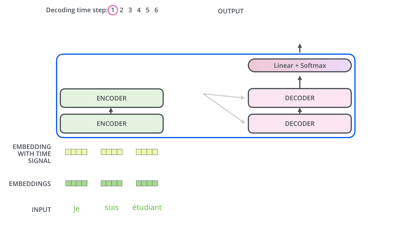
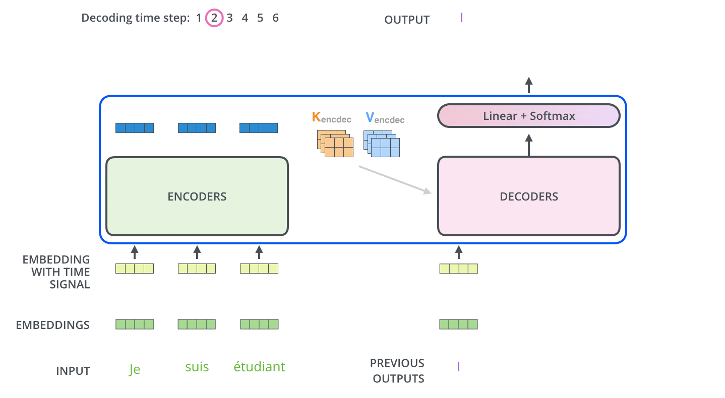
Transformer Architecture
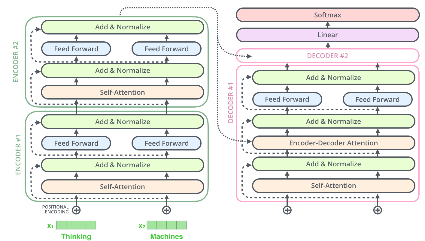
The Transformer using stacked self-attention and point-wise, fully connected layers for both the encoder and decoder, shown in the left and right halves of the following left figure, respectively.
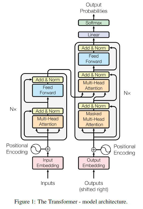
Encoder和Decoder均由6个layer堆叠组成:
Google AI Blog给出的动态展示过程

Encoder
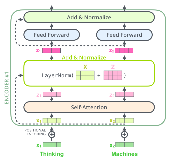
Encoder的layer由两个sublayer组成:multi-head self-attention和feed-forward network,两层sublayer均使用layer normalization和residual connection.
Encoder的输入层(最底层)需要做positional encoding,以考虑序列位置信息。所有层均需要做padding mask,以忽略padding的token。
FFN有两层,第一层是ReLU激活函数,第二层是线性激活函数,FFN可表示为
Tensorflow实现
class EncoderLayer(tf.keras.layers.Layer):
    """
    Each encoder layer consists of sublayers.
        1. Multi-head attention (with padding mask)
        2. Point wise feed forward networks.

    Each of these sublayers has a residual connection around it followed by a layer
    normalization. Residual connections help in avoiding the vanishing gradient problem
    in deep networks.
    """

    def __init__(self, d_model, num_heads, dff, rate=0.1):
        super(EncoderLayer, self).__init__()

        self.mha = MultiHeadAttention(d_model, num_heads)
        self.ffn = point_wise_feed_forward_network(d_model, dff)

        self.layernorm1 = tf.keras.layers.LayerNormalization(epsilon=1e-6)
        self.layernorm2 = tf.keras.layers.LayerNormalization(epsilon=1e-6)

        self.dropout1 = tf.keras.layers.Dropout(rate)
        self.dropout2 = tf.keras.layers.Dropout(rate)

    def call(self, x, training, mask):
        # all the shape=(batch_size, seq_len)
        attention_output, _ = self.mha(x, x, x, mask)
        attention_output = self.dropout1(attention_output, training=training)
        output1 = self.layernorm1(x + attention_output)

        ffn_output = self.ffn(output1)
        ffn_output = self.dropout2(ffn_output, training=training)
        output2 = self.layernorm2(output1 + ffn_output)
        return output2


class Encoder(tf.keras.layers.Layer):

    def __init__(self, num_layers, d_model, num_heads, dff, vocab_size, maximum_position_encoding,
                 rate=0.1):
        super(Encoder, self).__init__()

        self.d_model = d_model
        self.num_layers = num_layers
        self.embedding = tf.keras.layers.Embedding(vocab_size, d_model)
        self.pos_encoding = positional_encoding(maximum_position_encoding, d_model)
        self.enc_layers = [
            EncoderLayer(d_model, num_heads, dff, rate) for _ in range(num_layers)]
        self.dropout = tf.keras.layers.Dropout(rate)

    def call(self, x, training, mask):
        x = self.embedding(x)
        x *= tf.math.sqrt(tf.cast(self.d_model, tf.float32))
        x += self.pos_encoding[:, :tf.shape(x)[1], :]
        x = self.dropout(x, training=training)
        for enc_layer in self.enc_layers:
            x = enc_layer(x, training, mask)
        return x
Why does embedding vector multiplied by a constant in Transformer model? 词向量在加上位置嵌入之前,通过乘以常数(词向量维度的根号)进行放大,可能是想尽量保留语义信息,避免添加位置嵌入后语义信息丢失。此外,在self-attention中计算执行softmax计算分数概率分布时,也会除以这个常数!
x *= tf.math.sqrt(tf.cast(self.d_model, tf.float32))
Decoder
Decoder的layer由三个sublayer组成:
- Masked multi-head attention (with look ahead mask and padding mask);
- Masked multi-head attention (with padding mask). V and K receive the encoder outputs as inputs, Q receives the output from the first multi-head sublayer;
- Point wise feed forward networks;
解码器第一层multi-head除使用padding mask、positional encoding之外,还对使用look ahead mask,约束当前解码不考虑未来的信息。
解码器二层multi-head使用第一层multi-head的输出作为Q向量,K和V向量来自于Encoder,保证每次解码时考虑全部输入信息。
解码器第三层与编码器一致,使用FFN输出。解码器的不同sublayer间,同样使用residual connection和layer normalization。
Tensorflow实现
class DecoderLayer(tf.keras.layers.Layer):
    def __init__(self, d_model, num_heads, dff, rate=0.1):
        super(DecoderLayer, self).__init__()

        self.mha1 = MultiHeadAttention(d_model, num_heads)
        self.mha2 = MultiHeadAttention(d_model, num_heads)
        self.ffn = point_wise_feed_forward_network(d_model, dff)

        self.layernorm1 = tf.keras.layers.LayerNormalization(epsilon=1e-6)
        self.layernorm2 = tf.keras.layers.LayerNormalization(epsilon=1e-6)
        self.layernorm3 = tf.keras.layers.LayerNormalization(epsilon=1e-6)

        self.dropout1 = tf.keras.layers.Dropout(rate)
        self.dropout2 = tf.keras.layers.Dropout(rate)
        self.dropout3 = tf.keras.layers.Dropout(rate)

    def call(self, x, enc_output, training, combined_mask, enc_mask):
        attn1, block1 = self.mha1(x, x, x, combined_mask)
        attn1 = self.dropout1(attn1, training=training)
        out1 = self.layernorm1(attn1 + x)

        attn2, block2 = self.mha2(enc_output, enc_output, out1, enc_mask)
        attn2 = self.dropout2(attn2, training=training)
        out2 = self.layernorm2(attn2 + out1)

        ffn_output = self.ffn(out2)
        ffn_output = self.dropout3(ffn_output, training=training)
        out3 = self.layernorm3(ffn_output + out2)
        return out3, block1, block2


class Decoder(tf.keras.layers.Layer):
    def __init__(self, num_layers, d_model, num_heads, dff, vocab_size, maximum_position_encoding,
                 rate=0.1):
        super(Decoder, self).__init__()

        self.d_model = d_model
        self.num_layers = num_layers
        self.embedding = tf.keras.layers.Embedding(vocab_size, d_model)
        self.pos_encoding = positional_encoding(maximum_position_encoding, d_model)
        self.dec_layers = [
            DecoderLayer(d_model, num_heads, dff, rate) for _ in range(num_layers)]
        self.dropout = tf.keras.layers.Dropout(rate)

    def call(self, x, enc_output, training, combined_mask, enc_mask):
        x = self.embedding(x)
        x *= tf.math.sqrt(tf.cast(self.d_model, tf.float32))
        x += self.pos_encoding[:, :tf.shape(x)[1], :]
        x = self.dropout(x, training=training)

        attention_weights = {}
        for i, dec_layer in enumerate(self.dec_layers):
            x, block1, block2 = dec_layer(x, enc_output, training, combined_mask, enc_mask)
            attention_weights['decoder_layer{}_block1'.format(i + 1)] = block1
            attention_weights['decoder_layer{}_block2'.format(i + 1)] = block2

        return x, attention_weights
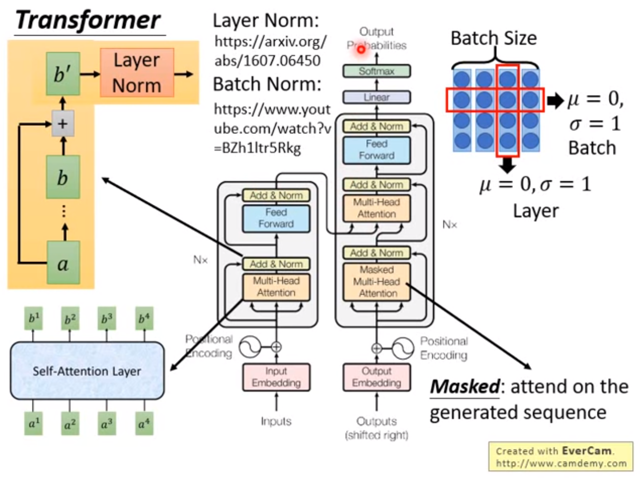
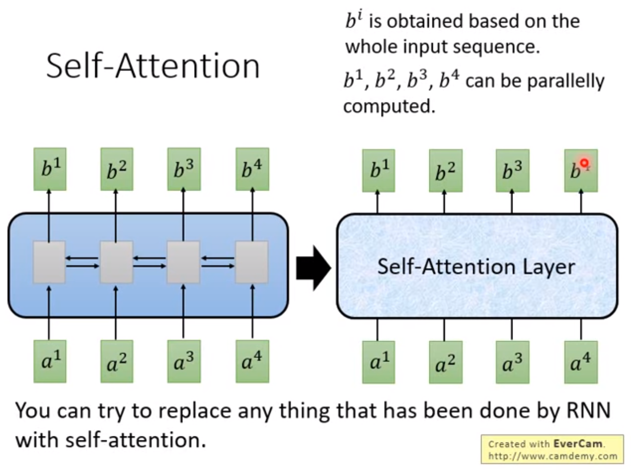
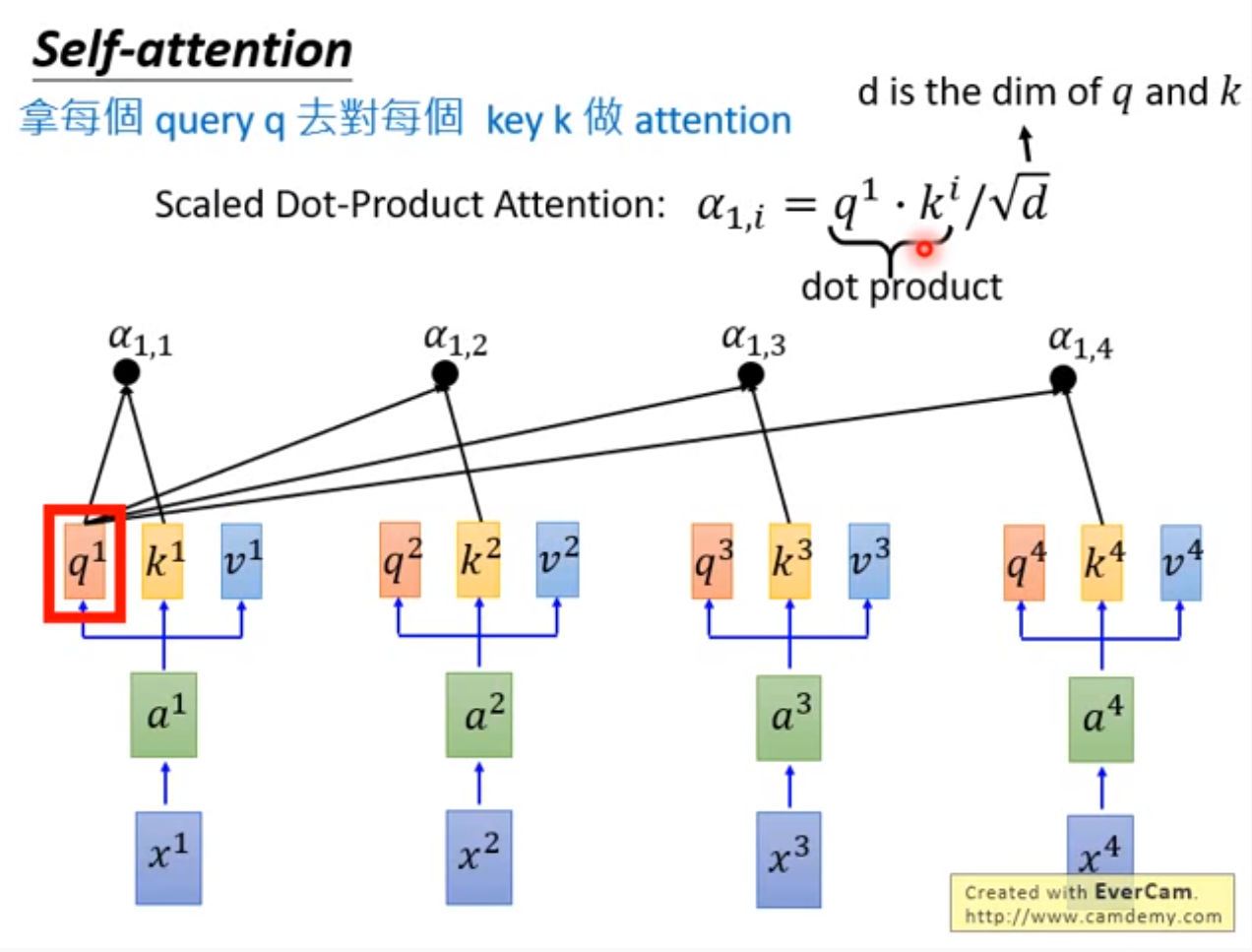
Self Attention
The rnn-model does not support parallel computing, self-attention layer is designed for address the problem.
Self-attention have two kind of forms: scaled dot-product attention and multi-head attention.
Scaled Dot-Product Attention

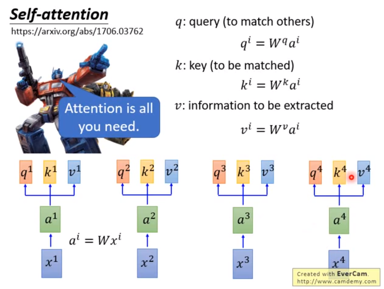
不同的输入向量 经线性变换矩阵 、 和 为查询向量 、键向量 和值向量 ,每个查询向量 与同序列其他输入的键向量 做内积,得到 将每个 作为输出的注意力/分数 。
对分数向量
使用softmax得到具有概率分布的分数,加权
得到
的输出向量
,计算公式如下
维度较高时内积值过大,softmax在较大值处的梯度较小,除以
避免梯度过小。
Transform each of input embedding to vector query , key , value by multiply the matrix on the left.
Take the scaled dot-product of each of and each of to get the value , and then normalizes it into a probability distribution with applying softmax, which is the attention of (output of ) on .
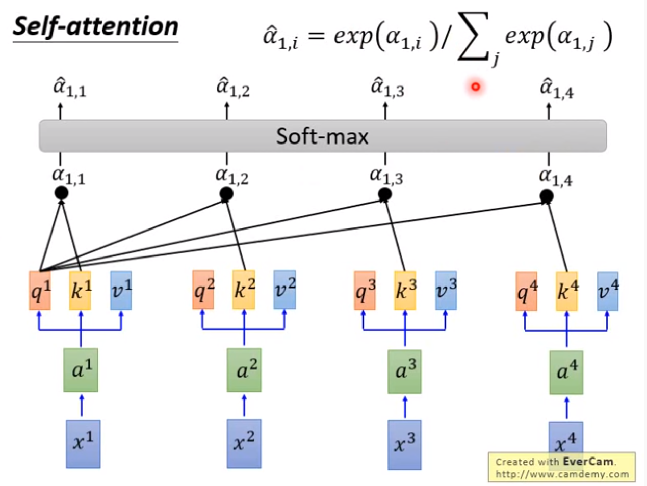
Matrix form of self-attention for parallel computing:
We suspect that for large values of
, the dot products grow large in magnitude, pushing the softmax function into regions where it has extremely small gradients. To counteract this effect, we scale the dot products by
. Maybe for small values of
, the scale is not necessary.
To illustrate why the dot products get large, assume that the components of and are independent random variables with mean 0 and variance 1. Then their dot product, has mean 0 and variance .
Tensorflow实现
def scaled_dot_product_attention(q, k, v, mask):
    """
    The transformer takes three inputs: Q (query), K (key), V (value).

    The equation used to calculate the attention weights is:
        Attention(Q, K, V) = softmax(Q·K^T/sqrt(d_k))V

    sqrt(d_k): This is done because for large valus of depth, the dot product grows large
    in magnitude pushing the softmax function where it has small gradients resulting in a
    very hard softmax.

    The mask is multiplied with 1e-9 (close to negative infinity), and large negative
    inputs to softmax are near zero in the output.

    :param q: shape=(..., seq_len, depth)
    :param k: shape=(..., seq_len, depth)
    :param v: shape=(..., seq_len, depth_v)
    :param mask: shape=(..., seq_len, seq_len)
        multi_head => (batch_size, 1, 1, seq_len), 利用广播性质mask
    """
    # (..., seq_len, seq_len)
    matmul_qk = tf.matmul(q, k, transpose_b=True)
    dk = tf.cast(tf.shape(k)[-1], tf.float32)
    scaled_attention_logits = matmul_qk / tf.math.sqrt(dk)

    if mask is not None:
        # padding_mask = (batch_size, 1, 1, seq_len)
        # combined_mask = (batch_size, 1, seq_len, seq_len)
        scaled_attention_logits += (mask * -1e9)

    # softmax is normalized on the last axis (seq_len) so that the scores add up to 1.
    # (..., seq_len, seq_len), 对最后二维矩阵的行做归一化
    attention_weights = tf.nn.softmax(scaled_attention_logits, axis=-1)
    # (..., seq_len, depth_v)
    output = tf.matmul(attention_weights, v)

    return output, attention_weights
Multi-Head Attention
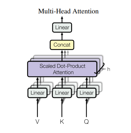
Multi-head attention consists of four parts:
-
Linear layers and split into heads.
-
Scaled dot-product attention.
-
Concatenation of heads.
-
Final linear layer.
Instead of one single attention head, Q, K, and V are split into multiple heads because it allows the model to jointly attend to information at different positions from different representational spaces.
Where the projections are parameter matrices:
If we employ
parallel attention layers, or heads, and use
. Due to the reduced dimension of each head, the total computational cost is similar to that of single-head attention with full dimensionality.
“多头” 模型可以分工关注序列内的局部或全局关联关系,效果很大可能优于同等计算量的 “单头” 模型。
Tensorflow实现
class MultiHeadAttention(tf.keras.layers.Layer):
    def __init__(self, d_model, num_heads):
        super(MultiHeadAttention, self).__init__()
        # number of scaled dot-product attentions
        self.num_heads = num_heads
        # dimension of output
        self.d_model = d_model
        assert d_model % num_heads == 0
        self.depth = d_model // num_heads
        self.wq = tf.keras.layers.Dense(d_model)
        self.wk = tf.keras.layers.Dense(d_model)
        self.wv = tf.keras.layers.Dense(d_model)
        self.dense = tf.keras.layers.Dense(d_model)

    def split_heads(self, x, batch_size):
        x = tf.reshape(x, (batch_size, -1, self.num_heads, self.depth))
        # 转置变换使得后期计算可以充分利用“广播”性质,加速计算
        return tf.transpose(x, perm=[0, 2, 1, 3])

    def call(self, v, k=None, q=None, mask=None):
        batch_size = tf.shape(q)[0]
        # shape=(batch_size, num_heads, seq_len, depth)
        q = self.split_heads(self.wq(q), batch_size)
        k = self.split_heads(self.wk(k), batch_size)
        v = self.split_heads(self.wv(v), batch_size)

        # scaled_attention.shape=(batch_size, num_heads, seq_len_q, depth)
        # attention_weights.shape=(batch_size, num_heads, seq_len_q, seq_len_k)
        scaled_attention, attention_weights = scaled_dot_product_attention(q, k, v, mask)
        # (batch_size, seq_len_q, num_heads, depth)
        scaled_attention = tf.transpose(scaled_attention, perm=[0, 2, 1, 3])
        # (batch_size, seq_len_q, d_model), d_model=num_heads*depth
        concat_attention = tf.reshape(scaled_attention, (batch_size, -1, self.d_model))

        # W_O matrix, (batch_size, seq_len_q, d_model)
        output = self.dense(concat_attention)
        return output, attention_weights
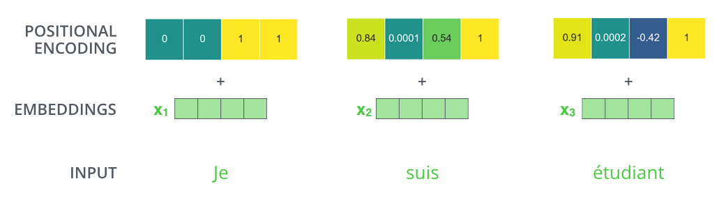
Positional Encoding
Since this model doesn’t contain any recurrence or convolution, positional encoding for giving the model some information about the relative position of the words in the sentence.
CNN和RNN得到的结果具有位置信息!
The intuition here is that adding these values to the embedding provides meaningful distances between the embedding vectors once they’re projected into Q/K/V vectors and during dot-product attention.
Positional encoding target: We can add a positional encoding vector to the embedding with d-dimension, after adding the positional encoding vector, words will be closer to each other based on the similarity of their meaning and their position in the sentence, in the d-dimensional space.
词嵌入添置位置嵌入后,空间距离越近的词距离越相近。
We use sine and cosine functions of different frequencies:
where is the position and is the dimension.
The following figure is positional encoding matrix with 50 length, 500 dimensions.
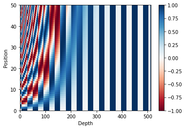
If the embedding has a dimensionality of 4, the actual positional encodings would look like this:
This is not the only possible method for positional encoding. It, however, gives the advantage of being able to scale to unseen lengths of sequences (e.g. if our trained model is asked to translate a sentence longer than any of those in our training set).
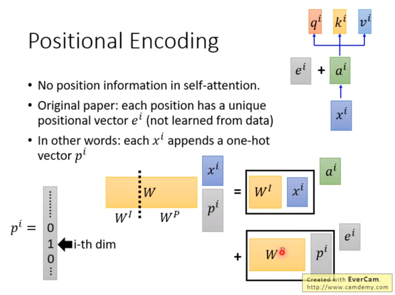
In other words, embedding vector
plus a constant vector
is equivalent to extend its dimension with a one hot vector.

Tensorflow实现
def positional_encoding(position, d_model):
    """
    Positional encoding is added to give the model some information about the relative
    position of the words in the sentence.

    The formula for calculating the positional encoding is as follwing:
        PE(pos,2i)   = sin(pos/10000^(2i/d_model))
        PE(pos,2i+1) = cos(pos/10000^(2i/d_model))
    """
    positions = np.arange(position)[:, np.newaxis]
    evens = np.arange(d_model)[np.newaxis, :] // 2
    angle_rates = 1 / np.power(10000, 2 * evens / np.float32(d_model))
    # shape=(seq_len, n_dimension)
    angle_rads = positions * angle_rates
    # even positions
    angle_rads[:, 0::2] = np.sin(angle_rads[:, 0::2])
    # odd position
    angle_rads[:, 1::2] = np.cos(angle_rads[:, 1::2])
    # shape=(1, position, n_dimension)
    encoding = angle_rads[np.newaxis, ...]
    return tf.cast(encoding, dtype=tf.float32)
Mask
mask表示掩码,是对某些值进行掩盖,使其在参数更新是不产生效果。
Transformer涉及padding mask和sequence mask/look ahead mask。 padding mask 在所有的 scaled dot-product attention里面都需要用到,而sequence mask只在decoder的 self-attention里面用到,decoder的输入层需同时考虑padding mask和sequence mask,给它取个新的名字combined mask。
Padding Mask: 由于各样本输入序列长度不一,需要对输入序列对齐至固定长度,如较短的序列填充0、较长的序列截断,在编解码时应当忽略这些padding位置。
Sequence mask: 解码器在时刻t解码时,为使解码器此时不考虑时刻t之后的状态,需要将t之后信息隐藏。具体做法是,产生维度等于序列长度、对角线元素为0的上三角矩阵,乘以大负数作用到attention权重,经过softmax后,模型在这些位置的注意力接近于0。
if mask is not None:
    # padding_mask = (batch_size, 1, 1, seq_len)
    # combined_mask = (batch_size, 1, seq_len, seq_len)
    scaled_attention_logits += (mask * -1e9)
Tensorflow实现
def create_padding_mask(sequence):
    """
    Mask all the pad tokens in the batch of sequence.
    It ensures that the model does not treat padding as the input.
    """
    # shape=(batch_size, seq_len)
    mask = tf.cast(tf.math.equal(sequence, 0), tf.float32)
    # shape=(batch_size, 1, 1, seq_len)
    mask = mask[:, tf.newaxis, tf.newaxis, :]
    return mask


def create_look_ahead_mask(size):
    """
    Mask the future tokens in a sequence. Used for decoding that mean the current output
    of decoder is independent of the future output.
    """
    # upper triangular matrix, shape=(seq_len, seq_len)
    mask = 1 - tf.linalg.band_part(tf.ones((size, size)), -1, 0)
    return mask


def create_combined_mask(sequence):
    """
    创建联合掩码
    主要用于解码器输入,需同时考虑padding_mask和look_ahead_mask
    """
    look_ahead_mask = create_look_ahead_mask(tf.shape(sequence)[1])
    padding_mask = create_padding_mask(sequence)
    combined_mask = tf.maximum(padding_mask, look_ahead_mask)
    return combined_mask
Layer Normalization
深度学习:层标准化详解(Layer Normalization)
Residual Connection/Skip Connection
There is a residual connection between each sub-layer (self-attention, ffnn), and is followed by a layer-normalization step. The layer norm output is:
The vectors and the layer-norm operation associated with self attention like:
"Residual Connections" is very important in retaining the position related information which we are adding to the input representation/embedding across the network.
Experimentally, the residual connections can be mainly applied to the concatenated positional encoding section to propagate it through, by concatenating positional encoding, instead of adding them, to the embedding.
通过将位置嵌入以扩展形式取代加性形式附加到词嵌入证明,Transformer中残差连接的主要作用是传播位置信息。
Residual Connection在梯度更新中的作用
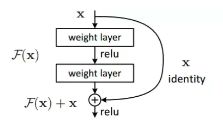
使用residual连接的层,对 求偏导时增加了一项常数项,有较大梯度更新 ,避免梯度消失。
Warm-Up Strategy and Post-LN Transformer
Adam优化器学习率的warm-up:
当total_steps=40000,warmup_steps=4000,学习率变化曲线:
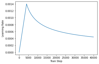
- 减缓模型初始阶段对mini-batch的提前过拟合现象,保持分布平稳
- 保持模型深度稳定性
- 训练时间增加
原始Transformer的layer norm放在residua过程之后,这种连接称为Post-LN Transformer. Post-LN Transformer对参数敏感,调参困难,必备warm-up学习策略,限制初始学习速率。
为什么需要限制模型初始学习速率?Post-LN Transformer训练初始阶段,输出层附近梯度非常大,初始阶段不加以限制学习率,模型学习可能爆炸。如果将layer-norm放在residual过程之中呢?这种连接称为Pre-LN Transformer,发现初始训练梯度下降很多,甚至不需要warm-up。

具体说明见Transformer中warm-up和LayerNorm的重要性探究。
Reference
1. Attention Is All You Need
2. The Illustrated Transformer–Jay Alammar
3. Transformer Architecture: Attention Is All You Need
4. Transformer中warm-up和LayerNorm的重要性探究
5.Transformer model for language understanding