Python实现简单的线性回归

最小二乘法实现

完整代码

from matplotlib import pyplot as plt
from pandas import Series, DataFrame

# 创建数据集
examDict = {'x': [0.50, 0.75, 1.00, 1.25, 1.50, 1.75, 1.75,
                     2.00, 2.25, 2.50, 2.75, 3.00, 3.25, 3.50, 4.00, 4.25, 4.50, 4.75, 5.00, 5.50],
            'y': [10, 22, 13, 43, 20, 22, 33, 50, 62,
                   48, 55, 75, 62, 73, 81, 76, 64, 82, 90, 93]}

# 转换为DataFrame的数据格式
examDf = DataFrame(examDict)
x=examDf.x
y=examDf.y
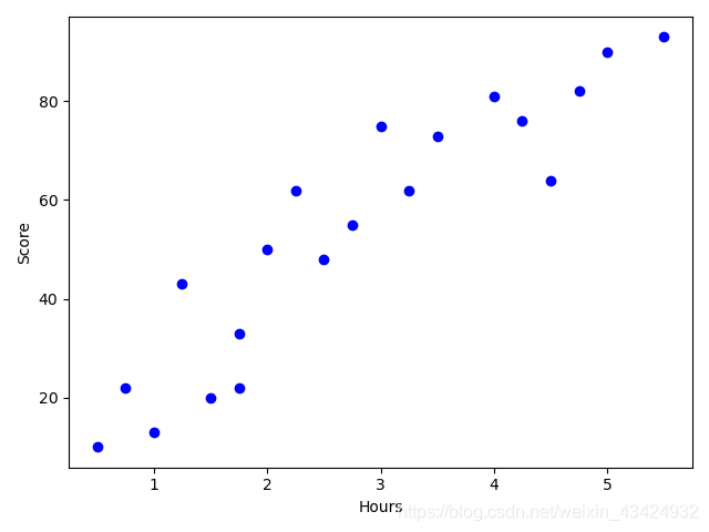
# 绘制散点图
plt.scatter(x, y, color='b', label="Exam Data")

# 添加图的标签（x轴，y轴）
plt.xlabel("Hours")
plt.ylabel("Score")
# 显示图像
plt.show()

# 损失函数
def cost(w,b,x,y):
    total_cost=0
    M=len(x)
    for i in range(M):
        total_cost+=(y[i]-w*x[i]-b)**2

    return total_cost/M

# 求平均数
def average(data):
    sum=0
    num=len(data)
    for i in range(num):
        sum+=data[i]
    return sum/num

# 求取w和b 
# 直线： y=w*x + b
def fit(x,y):
    M=len(x)
    x_bar= average(x)
    sum_yx=0
    sum_x2=0
    sum_delta=0
    for i in range(M):
        sum_yx+=y[i]*(x[i]-x_bar)
        sum_x2+=x[i]**2

    w=sum_yx/(sum_x2-M*(x_bar**2))

    for i in  range(M):
        sum_delta+=(y[i]-w*x[i])

    b=sum_delta/M

    return w,b
    

w,b=fit(x,y)
print("w is:",w)
print("b is:",b)
cost = cost(w,b,x,y)
print("cost is:",cost)

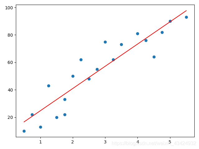
plt.scatter(x, y)
# 预测的y
pred_y=w*x +b
plt.plot(x,pred_y, color='r')
plt.show()

初始散点图

拟合效果图

梯度下降法实现

from matplotlib import pyplot as plt
from pandas import Series, DataFrame

# 创建数据集
examDict = {'x': [0.50, 0.75, 1.00, 1.25, 1.50, 1.75, 1.75,
                     2.00, 2.25, 2.50, 2.75, 3.00, 3.25, 3.50, 4.00, 4.25, 4.50, 4.75, 5.00, 5.50],
            'y': [10, 22, 13, 43, 20, 22, 33, 50, 62,
                   48, 55, 75, 62, 73, 81, 76, 64, 82, 90, 93]}

# 转换为DataFrame的数据格式
examDf = DataFrame(examDict)
x=examDf.x
y=examDf.y
# 绘制散点图
plt.scatter(x, y, color='b', label="Exam Data")

# 添加图的标签（x轴，y轴）
plt.xlabel("Hours")
plt.ylabel("Score")
# 显示图像
plt.show()

# 损失函数
def cost(w,b,x,y):
    total_cost=0
    M=len(x)
    for i in range(M):
        total_cost+=(y[i]-w*x[i]-b)**2

    return total_cost/M

alpha=0.001
initial_w=0
initail_b=0
num_iter=1000

# 算法
def grad_desc(x,y,initial_w,initail_b,alpha,num_iter):
    w=initial_w
    b=initail_b
    cost_list=[]
    for i in range(num_iter):
        cost_list.append(cost(w,b,x,y))
        w,b=step_grad_desc(w,b,alpha,x,y)
    return [w,b,cost_list]

def step_grad_desc(current_w,current_b,alpha,x,y):
    sum_grad_w=0
    sum_grad_b=0
    M=len(x)
    for i in range(M):
        sum_grad_w+=(current_w*x[i]+current_b-y[i])*x[i]
        sum_grad_b+=current_w*x[i]+current_b-y[i]

    gran_w=2/M*sum_grad_w
    grad_b=2/M*sum_grad_b

    update_w=current_w-alpha*gran_w
    update_b=current_b-alpha*grad_b

    return update_w,update_b

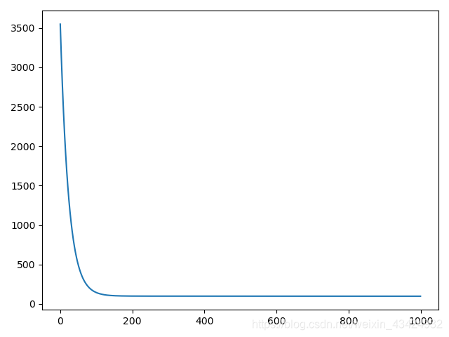
w,b,cost_list=grad_desc(x,y,initial_w,initail_b,alpha,num_iter)
print("w is:", w)
print("b is:", b)
print("cost is:",cost(w,b,x,y))
plt.plot(cost_list)
plt.show()

损失函数

拟合直线

调用sklearn实现

from sklearn.linear_model import LinearRegression
from matplotlib import pyplot as plt
from pandas import Series, DataFrame

# 创建数据集
examDict = {'x': [0.50, 0.75, 1.00, 1.25, 1.50, 1.75, 1.75,
                     2.00, 2.25, 2.50, 2.75, 3.00, 3.25, 3.50, 4.00, 4.25, 4.50, 4.75, 5.00, 5.50],
            'y': [10, 22, 13, 43, 20, 22, 33, 50, 62,
                   48, 55, 75, 62, 73, 81, 76, 64, 82, 90, 93]}

# 转换为DataFrame的数据格式
examDf = DataFrame(examDict)
x=examDf.x
y=examDf.y
# 绘制散点图
plt.scatter(x, y, color='b', label="Exam Data")

# 添加图的标签（x轴，y轴）
plt.xlabel("Hours")
plt.ylabel("Score")
# 显示散点图像
plt.show()

# 损失函数
def cost(w,b,x,y):
    total_cost=0
    M=len(x)
    for i in range(M):
        total_cost+=(y[i]-w*x[i]-b)**2

    return total_cost/M

# 调库
lr=LinearRegression()
lr.fit(x.values.reshape(-1, 1),y.values.reshape(-1, 1))

w=lr.coef_[0][0]
b=lr.intercept_[0]
print("w is:", w)
print("b is:", b)
cost=cost(w,b,x,y)
print("cost is:",cost)
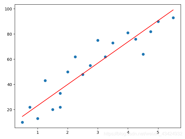
plt.scatter(x, y)
# 预测的y
pred_y=w*x +b
plt.plot(x,pred_y, color='r')
plt.show()

拟合直线