Python【线性回归】代码实现

一元线性回归

方法1：numpy

import numpy as np, matplotlib.pyplot as mp
# 数据
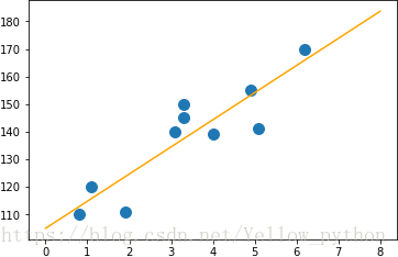
xp = [0.8, 1.1, 1.9, 3.1, 3.3, 3.3, 4.0, 5.1, 4.9, 6.2]
yp = [110, 120, 111, 140, 150, 145, 139, 141, 155, 170]
# 斜率、截距
k, b = np.polyfit(xp, yp, 1)
print(k, b)
# 可视化
xl = np.linspace(0, 8, 3)
yl = xl * k + b
mp.scatter(xp, yp, s=99)
mp.plot(xl, yl, color='orange')
mp.show()

方法2：sklearn

from sklearn import linear_model
import numpy as np, matplotlib.pyplot as mp
# 数据
x = [0.8, 1.1, 1.9, 3.1, 3.3, 3.3, 4.0, 5.1, 4.9, 6.2]
y = [110, 120, 111, 140, 150, 145, 139, 141, 155, 170]
x = np.array(x).reshape(-1, 1)
print(x)
# 建立线性回归模型
model = linear_model.LinearRegression()
# 拟合
model.fit(x, y)
# 斜率、截距
print(model.coef_, model.intercept_)
# 可视化
xl = np.array([0, 7]).reshape(-1, 1)
yl = model.predict(xl)  # 拟合方程
mp.scatter(x, y)
mp.plot(xl, yl, color='orange')
mp.show()

多元线性回归

import requests, re, pandas as pd, numpy as np, matplotlib.pyplot as mp
from mpl_toolkits import mplot3d  # 绘制3d图
from sklearn import linear_model
# 读数据-----------------------------------------------------------------
def download():
    url = 'https://blog.csdn.net/Yellow_python/article/details/81224614'
    header = {'User-Agent': 'Opera/8.0 (Windows NT 5.1; U; en)'}
    r = requests.get(url, headers=header)
    data = re.findall('<pre><code>([\s\S]+?)</code></pre>', r.text)[0].strip()
    df = pd.DataFrame([i.split(',') for i in data.split()], columns=['x1', 'x2', 'y'])
    df['x1'] = pd.to_numeric(df['x1'])
    df['x2'] = pd.to_numeric(df['x2'])
    df['y'] = pd.to_numeric(df['y'])
    return df
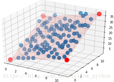
df = download()
# 线性回归-----------------------------------------------------------------
# 建立线性回归模型
model = linear_model.LinearRegression()
# 拟合
model.fit(df[['x1', 'x2']], df.y)
# 平面的系数、截距
k, b = model.coef_, model.intercept_
print(k, b)
# 给出待预测的特征（4个），并求得预测值
predict_x = pd.DataFrame([[0, 0], [0, 11], [11, 0], [11, 11]])
predict_y = predict_x[0] * k[0] + predict_x[1] * k[1] + b
# 拟合平面
x1, x2 = np.meshgrid(predict_x[0], predict_x[1])
y = x1 * k[0] + x2 * k[1] + b
# 可视化-----------------------------------------------------------------
fig = mp.figure()
ax = mplot3d.Axes3D(fig)  # 获取三维坐标轴
# 真实数据
ax.scatter(df.x1, df.x2, df.y, s=150)
# 预测数据
ax.scatter(predict_x[0], predict_x[1], predict_y, color='red', s=200)
# 拟合平面
ax.plot_surface(x1, x2, y, alpha=0.04, color='red')
mp.show()

附录：数据源

1,1,3.29
2,1,4.03
3,1,5.12
4,1,6.09
5,1,11.50
6,1,13.74
7,1,10.88
8,1,10.85
9,1,11.24
10,1,13.37
1,2,13.43
2,2,6.68
3,2,14.55
4,2,14.33
5,2,12.97
6,2,14.12
7,2,12.48
8,2,12.08
9,2,19.16
10,2,15.11
1,3,8.23
2,3,8.22
3,3,9.68
4,3,11.33
5,3,13.93
6,3,14.05
7,3,13.34
8,3,17.64
9,3,22.11
10,3,16.00
1,4,15.08
2,4,16.95
3,4,11.46
4,4,13.69
5,4,14.43
6,4,18.91
7,4,17.64
8,4,17.11
9,4,17.15
10,4,22.94
1,5,11.39
2,5,13.58
3,5,22.40
4,5,14.18
5,5,19.62
6,5,23.35
7,5,21.42
8,5,18.73
9,5,20.04
10,5,20.07
1,6,14.77
2,6,22.42
3,6,16.63
4,6,17.98
5,6,20.95
6,6,20.53
7,6,22.16
8,6,22.19
9,6,25.10
10,6,23.90
1,7,15.43
2,7,16.10
3,7,23.87
4,7,23.38
5,7,27.56
6,7,24.89
7,7,26.38
8,7,28.94
9,7,23.83
10,7,31.77
1,8,26.67
2,8,25.21
3,8,19.63
4,8,20.75
5,8,23.24
6,8,26.34
7,8,23.44
8,8,26.45
9,8,29.54
10,8,30.71
1,9,21.37
2,9,25.12
3,9,21.68
4,9,22.28
5,9,24.68
6,9,25.91
7,9,26.09
8,9,30.43
9,9,36.57
10,9,28.16
1,10,21.95
2,10,26.82
3,10,30.76
4,10,25.43
5,10,29.23
6,10,28.23
7,10,27.10
8,10,36.81
9,10,36.86
10,10,33.03