线性回归python实现

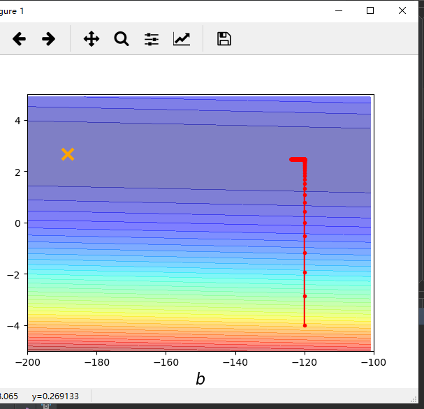
import numpy as np
import matplotlib.pyplot as plt

x_data = [338,333,328,207,226,25,179,60,208,606]
y_data = [640,633,619,393,428,27,193,66,226,1591]


#生成从-200到-100的数,不包括-100
#x轴
x = np.arange(-200,-100,1)
#y轴
y = np.arange(-5,5,0.1)
#存储对应的误差
Z = np.zeros((len(x),len(y)))
#x横向平铺给X,y纵向平铺给Y
#X,Y = np.meshgrid(x,y)
for i in range(len(x)):
    for j in range(len(y)):
        b = x[i]
        w = y[j]
        #按行进行计算误差
        Z[j][i] = 0
        #误差和
        for n in range(len(x_data)):
            Z[j][i] = Z[j][i] + (y_data[n] - b - w*x_data[n])**2
        #归一化
        Z[j][i] = Z[j][i]/len(x_data)


#y = b + w * x
b = -120
w = -4
lr = 0.0000001
iteration = 100000

b_history = [b]
w_history = [w]

for i in range(iteration):
    b_grad = 0.0
    w_grad = 0.0

    for n in range(len(x_data)):
        b_grad = b_grad - 2.0*(y_data[n] - b - w*x_data[n])*1.0
        w_grad = w_grad - 2.0 * (y_data[n] - b - w * x_data[n]) * x_data[n]

    b = b - lr * b_grad
    w = w - lr * w_grad

    b_history.append(b)
    w_history.append(w)

plt.contourf(x, y, Z, 50, alpha=0.5, cmap=plt.get_cmap('jet'))
plt.plot([-188.4],[2.67],'x',ms=12,markeredgewidth=3,color='orange')
plt.plot(b_history,w_history,'o-',ms = 3,lw = 1.5,color = 'red')
plt.xlim(-200,-100)
plt.ylim(-5,5)
plt.xlabel(r'$b$',fontsize=16)
plt.ylabel(r'$w$',fontsize=16)
plt.show()