[CS231n Assignment #1] 简单图像分类器——Softmax线性分类器

作业介绍

• 作业主页：Assignment #1
• 作业目的：
  • 针对Softmax分类器，实现一个全向量化的 损失函数(loss function)
  • 实现损失函数的矢量化解析梯度（analytic gradient）
  • 用 数值梯度（numerical gradient） 检验解析梯度是否正确
  • 使用测试集（val set）调试学习率和正则化程度大小（ the learning rate and regularization）
  • 使用 SGD 更新策略 最优化我们的SVM损失函数
  • 可视化最后学习到的权重
• 官方给的示例代码：assigment #1 code

知识点简单回顾

多分类交叉熵损失 和SVM损失不一样的是其在计算交叉熵损失之前需要讲输出 归一化（即统一成一个概率分布），具体的函数表达式如下：
$Softmax(x)_i = \frac {e^{s_i}} {\sum_{j=1}^{C} e^{s_j}} \quad (i=1,...,C)$
即其表示是C类中每类的概率。然后才是我们对于每一样本的损失函数：
$L_i = -\log \frac {e^{s_{y_i}}} {\sum_{j=1}^{C} e^{s_j}}= -s_{y_i} + \log \sum_{j=1}^{C} e^{s_j}$
其中 $s_j = W^TX$ 中的第 $j$ 类概率,理论上正确分类 $s_{y_i}$ 应该是1。

在信息论中，我们期望的概率分布 P = [0,0,1,0,…,0] 即只有正确分类的概率为1
而我们预测的分布 Q = [0.1,0.2,…,0.01] 可能和 P 不匹配
则其差别可用交叉熵来衡量 $L(P,Q) = \sum -\log P_iQ_i$
可以证明，当 Q = P时，交叉熵才会最小。

Hint:
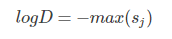
实际运算中，因为有指数运算，为了防止运算结果过大，所以我们需要进行处理进行处理：

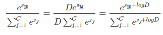
其中：

# python示例代码
scores = np.array([123, 456, 789])    # example with 3 classes and each having large scores
scores -= np.max(scores)    # scores becomes [-666, -333, 0]
p = np.exp(scores) / np.sum(np.exp(scores))

为了防止过拟合，我们还需要在最后的损失上加正则项。

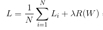
其中，

• 二范数正则使得权重尽可能均匀的小
• 一范数正则使得权重尽可能地稀疏，重点突出其中的几项
• $\lambda$ 越大，惩罚越大。同时也可能造成最后的概率分布更均匀，但是相对大小顺序不发生变化。

1. 下载数据集

参照之前的 KNN 分类器

2. Softmax分类器

• 使用 jupyter nodetebook 打开文件 softmax.ipynb 梳理一下流程（期间没有的python库需要自己手动安装一下）

2.1 加载图像并预处理

与之前的 svm一样，都需要减去均值图像。

2.2 实现损失函数

循环版

def softmax_loss_naive(W, X, y, reg):
  """
  Inputs:
  - W: A numpy array of shape (D, C) containing weights.
  - X: A numpy array of shape (N, D) containing a minibatch of data.
  - y: A numpy array of shape (N,) containing training labels; y[i] = c means
    that X[i] has label c, where 0 <= c < C.
  - reg: (float) regularization strength

  Returns a tuple of:
  - loss as single float
  - gradient with respect to weights W; an array of same shape as W
  """
  # Initialize the loss and gradient to zero.
  loss = 0.0
  dW = np.zeros_like(W)
  # 计算损失
  num_train = X.shape[0]
  num_class = W.shape[1]
  for i in range(num_train):
    # 计算得分
    scores = np.dot(X[i],W) # [1 , C]
    # 减去最大值，防止指数太大
    scores -= np.max(scores)
    # 指数并归一化
    correct_score = scores[y[i]]
    exp_scores_sum = np.sum(np.exp(scores))
    loss_i = -correct_score + np.log(exp_scores_sum) # 注意不写的时候np.log以e为底数
    loss += loss_i
    for j in range(num_class):
      softmax_output = np.exp(scores[j]) / exp_scores_sum
      if j == y[i]: # 正确类别的梯度
        dW[:,j] += (-1 + softmax_output) * X[i,:]
      else:
        dW[:,j] += softmax_output * X[i,:]
  loss /= num_train
  loss += 0.5 * reg * np.sum(W * W)
  dW /= num_train
  dW += reg * W

  return loss, dW

# 简单检查
from cs231n.classifiers.softmax import softmax_loss_naive
import time

# Generate a random softmax weight matrix and use it to compute the loss.
W = np.random.randn(3073, 10) * 0.0001
loss, grad = softmax_loss_naive(W, X_dev, y_dev, 0.0)

# As a rough sanity check, our loss should be something close to -log(0.1).
print('loss: %f' % loss)
print('sanity check: %f' % (-np.log(0.1)))

这里提出了 Question 1

向量化版

def softmax_loss_vectorized(W, X, y, reg):
  """
  Inputs:
  - W: A numpy array of shape (D, C) containing weights.
  - X: A numpy array of shape (N, D) containing a minibatch of data.
  - y: A numpy array of shape (N,) containing training labels; y[i] = c means
    that X[i] has label c, where 0 <= c < C.
  - reg: (float) regularization strength

  Returns a tuple of:
  - loss as single float
  - gradient with respect to weights W; an array of same shape as W
  """
  loss = 0.0
  dW = np.zeros_like(W)
  num_train = X.shape[0]
  num_class = W.shape[1]
  # 算出得分
  scores = np.dot(X,W) #[N,C]
  # 找出每行的最大值
  scores_max = np.max(scores,axis = 1,keepdims= True) # [N,1]
  # 减去最大值
  scores -= scores_max
  # 概率分布
  soft_max = np.exp(scores) / np.sum(np.exp(scores),axis = 1,keepdims = True) # [N , C]
  # 计算样本损失
  loss = np.sum(-np.log(soft_max[range(num_train),y])) # 之后正确类别才有交叉熵损失
  # 添加正则损失
  loss /= num_train
  loss += 0.5 * reg * np.sum(W * W)

  # 计算梯度
  dS = soft_max
  dS[range(num_train),y] -= 1 # 正确分类要减1
  dW = np.dot(X.T,dS)
  dW /= num_train
  dW += reg * W

2.3 使用随机梯度下降法优化

首先实现cs231n\classifiers\linear_classifier.py中的线性分类器LinearClassifier和Softmax分类部分。

class LinearClassifier(object):

    def __init__(self):
        self.W = None

    def train(self, X, y, learning_rate=1e-3, reg=1e-5, num_iters=100,
              batch_size=200, verbose=False):
        """
        Train this linear classifier using stochastic gradient descent.

        Inputs:
        - X: A numpy array of shape (N, D) containing training data; there are N
          training samples each of dimension D.
        - y: A numpy array of shape (N,) containing training labels; y[i] = c
          means that X[i] has label 0 <= c < C for C classes.
        - learning_rate: (float) learning rate for optimization.
        - reg: (float) regularization strength.
        - num_iters: (integer) number of steps to take when optimizing
        - batch_size: (integer) number of training examples to use at each step.
        - verbose: (boolean) If true, print progress during optimization.

        Outputs:
        A list containing the value of the loss function at each training iteration.
        """
        num_train, dim = X.shape
        num_classes = np.max(y) + 1 # assume y takes values 0...K-1 where K is number of classes
        if self.W is None:
            # lazily initialize W
            self.W = 0.001 * np.random.randn(dim, num_classes)

        # Run stochastic gradient descent to optimize W
        loss_history = []
        for it in range(num_iters):
            X_batch = None
            y_batch = None

            # 从 0 ~ num_train - 1 中随机选择 batch_size 个数
            # 问题不能讲样本取尽
            batch_indices = np.random.choice(num_train,batch_size,replace = True)
            X_batch = X[batch_indices]
            y_batch = y[batch_indices]

            # evaluate loss and gradient
            loss, grad = self.loss(X_batch, y_batch, reg)
            loss_history.append(loss)

            # Update the weights using the gradient and the learning rate.          #
            self.W -= learning_rate * grad

            if verbose and it % 100 == 0:
                print('iteration %d / %d: loss %f' % (it, num_iters, loss))

        return loss_history

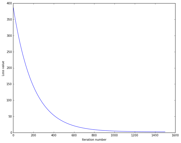
训练测试

from cs231n.classifiers import Softmax
softmax = Softmax()
tic = time.time()
loss_hist = softmax.train(X_train, y_train, learning_rate=1e-7, reg=2.5e4,
                      num_iters=1500, verbose=True)
toc = time.time()
print('That took %fs' % (toc - tic))

plt.plot(loss_hist)
plt.xlabel('Iteration number')
plt.ylabel('Loss value')
plt.show()

2.4 完成预测

• 其中 分类器的基类代码已经在 SVM Classifier 的时候完成了。

 def predict(self, X):
        """
        Use the trained weights of this linear classifier to predict labels for
        data points.
        Inputs:
        - X: A numpy array of shape (N, D) containing training data; there are N
          training samples each of dimension D.

        Returns:
        - y_pred: Predicted labels for the data in X. y_pred is a 1-dimensional
          array of length N, and each element is an integer giving the predicted
          class.
        """
        y_pred = np.zeros(X.shape[0])
        scores = np.dot(X,self.W)
        y_pred = np.argmax(scores,axis = 1) # 取出每一行最大得分类别
        return y_pred

y_train_pred = softmax.predict(X_train)
print('training accuracy: %f' % (np.mean(y_train == y_train_pred), ))
y_val_pred = softmax.predict(X_val)
print('validation accuracy: %f' % (np.mean(y_val == y_val_pred), ))

2.5 使用验证集调参

• 设置参数，例如学习率和正则化强度的变化范围
• 参数在指定范围内变化，然后计算其在验证集上的精度
• 选择多次验证后的最优参数，然后计算其在测试集上的性能

from cs231n.classifiers import Softmax
results = {}
best_val = -1
best_softmax = None
# 凭自己喜好，可以取少一点，测试快一点
learning_rates = [1.4e-7, 1.5e-7, 1.6e-7]
regularization_strengths = [8000.0, 9000.0, 10000.0, 11000.0, 18000.0, 19000.0, 20000.0, 21000.0]
best_lr = None
beat_reg = None

num_iters = 1000

for lr in learning_rates:
    for reg in regularization_strengths:
        softmax = Softmax()
        softmax.train(X_train,y_train,
                      learning_rate=lr,
                      reg = reg,
                     num_iters = num_iters)
        y_train_pred = softmax.predict(X_train)
        train_acc = np.mean(y_train == y_train_pred)
        y_val_pred = softmax.predict(X_val)
        val_acc = np.mean(y_val == y_val_pred)
        results[(lr,reg)] = (train_acc,val_acc)
        if val_acc > best_val:
            best_lr = lr
            best_reg = reg
            best_val = val_acc
            best_softmax = softmax
        
# Print out results.
for lr, reg in sorted(results):
    train_accuracy, val_accuracy = results[(lr, reg)]
    print('lr %e reg %e train accuracy: %f val accuracy: %f' % (
                lr, reg, train_accuracy, val_accuracy))
    
print('Best validation accuracy during cross-validation:\nlr = %e, reg = %e, best_val = %f' %
      (best_lr, best_reg, best_val)) 
plt.show()

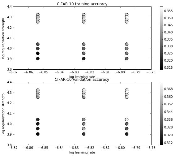
可视化每组参数的精度

import math
x_scatter = [math.log10(x[0]) for x in results]
y_scatter = [math.log10(x[1]) for x in results]

# plot training accuracy
marker_size = 100
colors = [results[x][0] for x in results]
plt.subplot(2, 1, 1)
plt.scatter(x_scatter, y_scatter, marker_size, c=colors)
plt.colorbar()
plt.xlabel('log learning rate')
plt.ylabel('log regularization strength')
plt.title('CIFAR-10 training accuracy')

# plot validation accuracy
colors = [results[x][1] for x in results] # default size of markers is 20
plt.subplot(2, 1, 2)
plt.scatter(x_scatter, y_scatter, marker_size, c=colors)
plt.colorbar()
plt.xlabel('log learning rate')
plt.ylabel('log regularization strength')
plt.title('CIFAR-10 validation accuracy')
plt.show()

测试在测试集上的精度

# evaluate on test set
# Evaluate the best softmax on test set
y_test_pred = best_softmax.predict(X_test)
test_accuracy = np.mean(y_test == y_test_pred)
print('softmax on raw pixels final test set accuracy: %f' % (test_accuracy, ))

这里给出了 Question 2

2.6 可视化权重

# Visualize the learned weights for each class
w = best_softmax.W[:-1,:] # strip out the bias
w = w.reshape(32, 32, 3, 10)

w_min, w_max = np.min(w), np.max(w)

classes = ['plane', 'car', 'bird', 'cat', 'deer', 'dog', 'frog', 'horse', 'ship', 'truck']
for i in range(10):
    plt.subplot(2, 5, i + 1)
    
    # Rescale the weights to be between 0 and 255
    wimg = 255.0 * (w[:, :, :, i].squeeze() - w_min) / (w_max - w_min)
    plt.imshow(wimg.astype('uint8'))
    plt.axis('off')
    plt.title(classes[i])

作业问题

• Q1: Why do we expect our loss to be close to -log(0.1)? Explain briefly.
• 即在初始完权重，检查损失的时候，为什么损失接近于 -log(0.1)
• A1: 因为我们初始化权重的时，权重值比较下，导致最后得到的各类的得分都比较小，进而归一化的概率比较接近，所以我们的损失之就接近于 $-\log \frac {1} {C}$。
• Q2： It’s possible to add a new datapoint to a training set that would leave the SVM loss unchanged, but this is not the case with the Softmax classifier loss.
• A2： 是可能的，因为SVM分类器只需要满足正确类别的得分比其它类别的值大就行了，但是softmax需要满足正确类别的得分概率归一化后需要是1，即除非它的正确类得分比其他类大很多很多，否则都不是0.所以，可以增加一个样本，其满足SVM中正确类别比其它类别的得分大，则SVM损失不增加，但是Softmax损失会有一定增加。

参考资料

• cs231n linear classification notes