[CS231n Assignment #1] 简单图像分类器——KNN分类器

文章目录

作业介绍
1. 下载数据集并加载
2. KNN(K近邻分类器)

2.1 加载数据集
2.2 完成我们的KNN分类器
2.3 测试KNN分类器

3. 多折交叉验证调优

作业介绍

作业主页：Assignment #1
作业目的：
- 理解图像分类流程和数据驱动方法（训练和预测阶段）
- 理解训练集(train dataset）、验证集(val dataset)、测试集(test dataset)的划分，以及验证集对于超参数的选择
- 学会用 numpy 库编写向量化代码
- 实现KNN、SVM、Softmax和两层神经网络分类器
- 理解不同分类器间的区别，和各自的权衡
- 理解用更高级的特征表达（例如颜色直方图，方向梯度特征HOG），而不是原始图像带来的分类器性能的提升
官方给的示例代码：assigment #1 code

1. 下载数据集并加载

两种方法下载：

cd 到路径 cs231n/datasets运行脚本get_datasets.sh，下载并解压
直接到 CIFAR10 官网上下载python版的数据集格式cifar-10-python.tar.gz，解压cifar-10-python然后放在当前路径的子路径./CIFAR10/datasets/下
最后的路径应该是cs231n/datasets/cifar-10-batches-py/6个批次

数据组织：

数据包含5个训练批次batch和一个测试批次
每个批次包含 10,000 * 3072 维度的矩阵，代表10000个32x32x3的RGB图片，同时也包含10000个标签，用字典存储data & labels
总的数据一共分为10类，类别用0~9表示，类别信息存储在batches.meta，包含一个字典label_names，第i类别名label_names[i]。

2. KNN(K近邻分类器)

使用 jupyter nodetebook 打开文件 knn.ipynb 梳理一下流程（期间没有的python库需要自己手动安装一下）

Setup Code
运行setup code设置notebook格式

# Run some setup code for this notebook.
import random
import numpy as np
from cs231n.data_utils import load_CIFAR10
import matplotlib.pyplot as plt

from __future__ import print_function

# This is a bit of magic to make matplotlib figures appear inline in the notebook
# rather than in a new window.
%matplotlib inline
plt.rcParams['figure.figsize'] = (10.0, 8.0) # set default size of plots
plt.rcParams['image.interpolation'] = 'nearest'
plt.rcParams['image.cmap'] = 'gray'

# Some more magic so that the notebook will reload external python modules;
# see http://stackoverflow.com/questions/1907993/autoreload-of-modules-in-ipython
%load_ext autoreload
%autoreload 2

2.1 加载数据集

Load the raw CIFAR-10 data

cifar10_dir = 'cs231n/datasets/cifar-10-batches-py' # 6个batch所在路径

# Cleaning up variables to prevent loading data multiple times (which may cause memory issue)
try:
   del X_train, y_train
   del X_test, y_test
   print('Clear previously loaded data.')
except:
   pass

X_train, y_train, X_test, y_test = load_CIFAR10(cifar10_dir)

# As a sanity check, we print out the size of the training and test data.
print('Training data shape: ', X_train.shape) # 50000 * 32 * 32 * 3
print('Training labels shape: ', y_train.shape) # 50000
print('Test data shape: ', X_test.shape) # 10000 * 32 * 32 * 3
print('Test labels shape: ', y_test.shape) # 10000

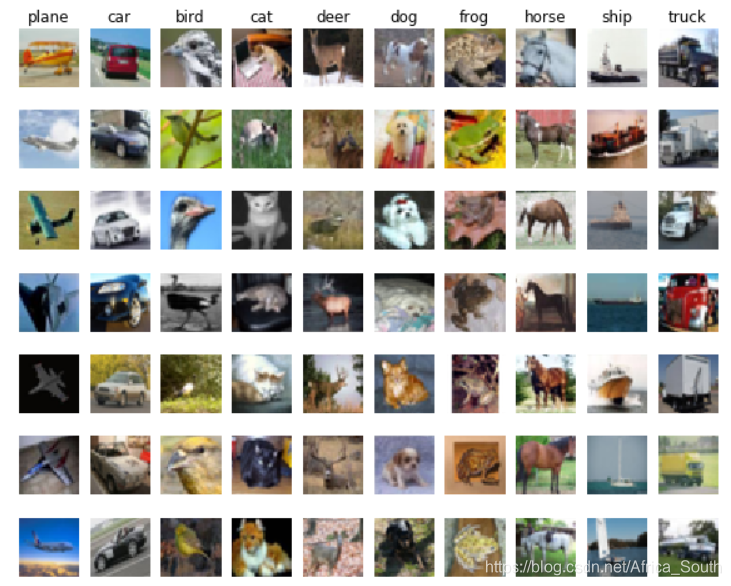
Visualize some examples

classes = ['plane', 'car', 'bird', 'cat', 'deer', 'dog', 'frog', 'horse', 'ship', 'truck']
num_classes = len(classes)
samples_per_class = 7
for y, cls in enumerate(classes):
    # np.flatnonzero() 输入一个矩阵然后返回其中非零元素的索引位置
    idxs = np.flatnonzero(y_train == y)
    # 随机采样
    idxs = np.random.choice(idxs, samples_per_class, replace=False)
    for i, idx in enumerate(idxs):
        # 在显示矩阵中的位置
        plt_idx = i * num_classes + y + 1
        plt.subplot(samples_per_class, num_classes, plt_idx)
        plt.imshow(X_train[idx].astype('uint8'))
        plt.axis('off')
        if i == 0:
            plt.title(cls)
plt.show()

在这里插入图片描述

Subsample the data for more efficient code execution in this exercise

# 从训练集和测试集中选出部分子集
# 代码技巧：可以先生成一个子集索引的掩码mask
num_training = 5000
mask = list(range(num_training))
X_train = X_train[mask]
y_train = y_train[mask]

num_test = 500
mask = list(range(num_test))
X_test = X_test[mask]
y_test = y_test[mask]

# 将 N*H*W*C -> N *(H*W*C)
# 即 5000 * 32 * 32 * 3 -> 5000 * 3072
X_train = np.reshape(X_train, (X_train.shape[0], -1))
X_test = np.reshape(X_test, (X_test.shape[0], -1))
print(X_train.shape, X_test.shape)

Test our KNN Classifier

from cs231n.classifiers import KNearestNeighbor

# Create a kNN classifier instance. 
# Remember that training a kNN classifier is a noop: 
# the Classifier simply remembers the data and does no further processing 
classifier = KNearestNeighbor()
classifier.train(X_train, y_train)

注意：这时候我们就需要先完成cs231n/classifiers/k_nearest_neighbor.py的编写

2.2 完成我们的KNN分类器

KNN分类器定义在cs231n/classifiers/k_nearest_neighbor.py

记住所有的训练数据和其标签
对于测试数据，选择K个和其距离（例如欧式距离或其它距离度量方式）最近的数据，选择这K个数据中代表标签最多的，就是测试数据的标签

# coding=UTF-8
import numpy as np

class KNearestNeighbor(object):
  """a KNN classifier with L2 distance"""
  def __init__(self):
    self.X_train = None
    self.y_train = None

  def train(self, X, y):
    """
    Train the classifier. For k-nearest neighbors this is just
    memorizing the training data.

    Inputs:
    - X: A numpy array of shape (num_train, D) containing the training data
      consisting of num_train samples each of dimension D.
    - y: A numpy array of shape (N,) containing the training labels, where
         y[i] is the label for X[i].
    """
    self.X_train = X
    self.y_train = y
    
  def predict(self, X, k=1, num_loops=0):
    """
    Predict labels for test data using this classifier.

    Inputs:
    - X: A numpy array of shape (num_test, D) containing test data consisting
         of num_test samples each of dimension D.
    - k: The number of nearest neighbors that vote for the predicted labels.
    - num_loops: Determines which implementation to use to compute distances
      between training points and testing points.

    Returns:
    - y: A numpy array of shape (num_test,) containing predicted labels for the
      test data, where y[i] is the predicted label for the test point X[i].  
    """
    if num_loops == 0:
      dists = self.compute_distances_no_loops(X)
    elif num_loops == 1:
      dists = self.compute_distances_one_loop(X)
    elif num_loops == 2:
      dists = self.compute_distances_two_loops(X)
    else:
      raise ValueError('Invalid value %d for num_loops' % num_loops)

    return self.predict_labels(dists, k=k)

  def compute_distances_two_loops(self, X):
    """
    Compute the distance between each test point in X and each training point
    in self.X_train using a nested loop over both the training data and the 
    test data.

    Inputs:
    - X: A numpy array of shape (num_test, D) containing test data.

    Returns:
    - dists: A numpy array of shape (num_test, num_train) where dists[i, j]
      is the Euclidean distance between the ith test point and the jth training
      point.
    """
    num_test = X.shape[0]
    num_train = self.X_train.shape[0]
    dists = np.zeros((num_test, num_train))
    for i in range(num_test):
      for j in range(num_train):
        # first compute (x_i - x_j) ^ 2
        # then sum them
        # finally sqrt
        dists[i,j] = np.sqrt(np.sum(np.square(X[i] - self.X_train[j])))
    return dists

  def compute_distances_one_loop(self, X):
    """
    Compute the distance between each test point in X and each training point
    in self.X_train using a single loop over the test data.

    Input / Output: Same as compute_distances_two_loops
    """
    num_test = X.shape[0]
    num_train = self.X_train.shape[0]
    dists = np.zeros((num_test, num_train))
    for i in range(num_test):
      # 利用 numpy 数组的广播机制
      dists[i] = np.sqrt(np.sum(np.square(X[i] - self.X_train),axis = 1))
    return dists

  def compute_distances_no_loops(self, X):
    """
    Compute the distance between each test point in X and each training point
    in self.X_train using no explicit loops.

    Input / Output: Same as compute_distances_two_loops
    """
    num_test = X.shape[0]
    num_train = self.X_train.shape[0]
    dists = np.zeros((num_test, num_train))
    # (X - X_train)*(X - X_train) = -2X*X_train + X*X + X_train*X_train
    # 假设测试集的维度是 [M,D]
    # 先计算测试集行向量组的平方
    d1 = np.sum(np.square(X),axis = 1,keepdims= True) # [M,1]
    # 再计算训练集行向量的平方
    d2 = np.sum(np.square(self.X_train),axis = 1) # [N,]
    # 再计算两个矩阵行向量组的乘积
    d3 = np.dot(X,self.X_train.T) # [M , N]
    # 最后计算结果
    # 会进行广播，注意d2广播时会在其维度浅先加一个1，变成[1,N]
    dists = np.sqrt(d1 - 2 * d3 + d2)
    return dists

  def predict_labels(self, dists, k=1):
    """
    Given a matrix of distances between test points and training points,
    predict a label for each test point.

    Inputs:
    - dists: A numpy array of shape (num_test, num_train) where dists[i, j]
      gives the distance betwen the ith test point and the jth training point.

    Returns:
    - y: A numpy array of shape (num_test,) containing predicted labels for the
      test data, where y[i] is the predicted label for the test point X[i].  
    """
    num_test = dists.shape[0]
    y_pred = np.zeros(num_test)
    for i in range(num_test):
      # A list of length k storing the labels of the k nearest neighbors to
      # the ith test point.
      closest_y = []
      # argsort(a, axis=-1, kind='quicksort', order=None)
      # 使用kind排序对a的axis维度进行排序，并返回排序后从小到大的值的索引
      sort_indices = np.sort(dists[i])
      sort_k = sort_indices[:k] # 取前k个最小的距离的索引
      # 找到前k个索引中标签最多的类别
      sort_labels = self.y_train[sort_k]
      y_pred[i] = np.argmax(np.bincount(sort_labels))
      # 注意这里没有考虑如果有两个标签的数目一样多该怎么办
    return y_pred

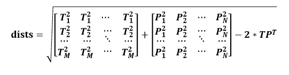
这里面稍微有点难度的就是矩阵间欧式距离的计算
假设测试集T的维度是 $M*D$ ，训练集P的维度是 $N * D$ ，即训练集有N个样本，测试集有M个样本，每个样本的维度是 D。
记 $T_i$ 是第 $i$ 个样本， $P_j$ 是训练集第 $j$ 个样本，则二者之间的距离：
在这里插入图片描述
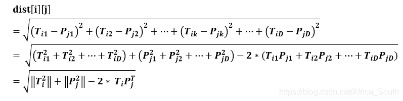
则我们任意两个测试样本和训练样本间的距离：

2.3 测试KNN分类器

from cs231n.classifiers import KNearestNeighbor

# Create a kNN classifier instance. 
# Remember that training a kNN classifier is a noop: 
# the Classifier simply remembers the data and does no further processing 
classifier = KNearestNeighbor()
classifier.train(X_train, y_train)

dists = classifier.compute_distances_two_loops(X_test)
print(dists.shape) # (500,5000)

plt.imshow(dists, interpolation='none')
plt.show()

# Now implement the function predict_labels and run the code below:
# We use k = 1 (which is Nearest Neighbor).
y_test_pred = classifier.predict_labels(dists, k=1)

# Compute and print the fraction of correctly predicted examples
num_correct = np.sum(y_test_pred == y_test)
accuracy = float(num_correct) / num_test
print('Got %d / %d correct => accuracy: %f' % (num_correct, num_test, accuracy))
# Got 137 / 500 correct => accuracy: 0.274000

y_test_pred = classifier.predict_labels(dists, k=5)
num_correct = np.sum(y_test_pred == y_test)
accuracy = float(num_correct) / num_test
print('Got %d / %d correct => accuracy: %f' % (num_correct, num_test, accuracy))
# Got 139 / 500 correct => accuracy: 0.278000

比较不同欧式距离计算方式的差别
结果差别：

# Now lets speed up distance matrix computation by using partial vectorization
# with one loop. Implement the function compute_distances_one_loop and run the
# code below:
dists_one = classifier.compute_distances_one_loop(X_test)

# To ensure that our vectorized implementation is correct, we make sure that it
# agrees with the naive implementation. There are many ways to decide whether
# two matrices are similar; one of the simplest is the Frobenius norm. In case
# you haven't seen it before, the Frobenius norm of two matrices is the square
# root of the squared sum of differences of all elements; in other words, reshape
# the matrices into vectors and compute the Euclidean distance between them.
difference = np.linalg.norm(dists - dists_one, ord='fro')
print('Difference was: %f' % (difference, ))
if difference < 0.001:
    print('Good! The distance matrices are the same')
else:
    print('Uh-oh! The distance matrices are different')

# Now implement the fully vectorized version inside compute_distances_no_loops
# and run the code
dists_two = classifier.compute_distances_no_loops(X_test)

# check that the distance matrix agrees with the one we computed before:
difference = np.linalg.norm(dists - dists_two, ord='fro')
print('Difference was: %f' % (difference, ))
if difference < 0.001:
    print('Good! The distance matrices are the same')
else:
    print('Uh-oh! The distance matrices are different')

时间花费

# Let's compare how fast the implementations are
def time_function(f, *args):
    """
    Call a function f with args and return the time (in seconds) that it took to execute.
    """
    import time
    tic = time.time()
    f(*args)
    toc = time.time()
    return toc - tic

two_loop_time = time_function(classifier.compute_distances_two_loops, X_test)
print('Two loop version took %f seconds' % two_loop_time)

one_loop_time = time_function(classifier.compute_distances_one_loop, X_test)
print('One loop version took %f seconds' % one_loop_time)

no_loop_time = time_function(classifier.compute_distances_no_loops, X_test)
print('No loop version took %f seconds' % no_loop_time)

# you should see significantly faster performance with the fully vectorized implementation

# 差别很大
# 而且惊讶的发现一次循环竟然比两次循环还慢
# 猜想可能是广播的时候还需要复制？？
Two loop version took 34.630000 seconds
One loop version took 120.321000 seconds
No loop version took 0.459000 seconds

3. 多折交叉验证调优

num_folds = 5
k_choices = [1, 3, 5, 8, 10, 12, 15, 20, 50, 100]

X_train_folds = []
y_train_folds = []

train_len = X_train.shape[0] # 获取训练数据的样本个数
fold_len = train_len / num_folds # 每一折的样本个数
for i in range(num_folds):
    # 多余的就省略不要
    X_train_folds.append(X_train[i*fold_len : (i+1) * fold_len])
    y_train_folds.append(y_train[i*fold_len : (i+1) * fold_len])
# 或者直接使用 numpy array_split function
# X_train_folds = np.split(X_train, num_folds)
# y_train_folds = np.split(y_train, num_folds)

# A dictionary holding the accuracies for different values of k that we find
# when running cross-validation. After running cross-validation,
# k_to_accuracies[k] should be a list of length num_folds giving the different
# accuracy values that we found when using that value of k.
k_to_accuracies = {}
for k in k_choices:
    # 对每个k进行一次实验
    accuracies = [] # 每一折的精度
    for j in range(num_folds):
        # 保留第 j 折作为测试集
        X_tr = np.concatenate(X_train_folds[0:j]+X_train_folds[j+1:])
        y_tr = np.concatenate(y_train_folds[0:j]+y_train_folds[j+1:])
        X_val = X_train_folds[j]
        y_val = y_train_folds[j]
        classifier.train(X_tr,y_tr)
        y_pre = classifier.predict(X_val,k=k,num_loops=0)
        accuracy = np.mean(y_pre == y_val)
        accuracies.append(accuracy) 
    k_to_accuracies[k] = accuracies # 每一个k都有,5折精度，是一个字典

# Print out the computed accuracies
for k in sorted(k_to_accuracies):
    for i in range(num_folds):
        print('k = %d, fold = %d, accuracy: %f' % (k, i+1, k_to_accuracies[k][i]))

画出精度线和误差线

# plot the raw observations
for k in k_choices:
    accuracies = k_to_accuracies[k]
    plt.scatter([k] * len(accuracies), accuracies)

# plot the trend line with error bars that correspond to standard deviation
accuracies_mean = np.array([np.mean(v) for k,v in sorted(k_to_accuracies.items())])
accuracies_std = np.array([np.std(v) for k,v in sorted(k_to_accuracies.items())])
plt.errorbar(k_choices, accuracies_mean, yerr=accuracies_std)
plt.title('Cross-validation on k')
plt.xlabel('k')
plt.ylabel('Cross-validation accuracy')
plt.show()

在这里插入图片描述
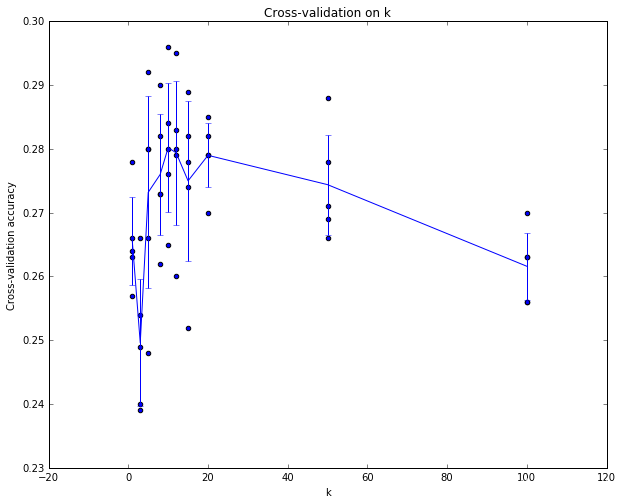
可以看到，每个k都对应于5个折的精度，然后我们取其平均值连起来，发现k=10左右精度比较高。

best_k = k_choices[np.argmax(accuracies_mean)]
print("the best k is %d" % best_k)
classifier = KNearestNeighbor()
classifier.train(X_train, y_train)
y_test_pred = classifier.predict(X_test, k=best_k)

# Compute and display the accuracy
num_correct = np.sum(y_test_pred == y_test)
accuracy = float(num_correct) / num_test
print('Got %d / %d correct => accuracy: %f' % (num_correct, num_test, accuracy))

the best k is 10
Got 141 / 500 correct => accuracy: 0.282000

灵隐寺扫地僧

发布了19 篇原创文章 · 获赞 1 · 访问量 507

私信关注