[CS231n Assignment #1] 简单图像分类器——单隐层神经网络分类器

作业介绍

• 作业主页：Assignment #1

• 官方给的示例代码：assigment #1 code

知识点简单回顾

神经网络(Neural Networks) 是一种非线性分类器，区别于 SVM分类器 和 Softmax分类器，它的中间网络层通过激活函数等手段引入了非线性性，而一个比较简单的网络模型如下，它只有一个中间隐藏层：

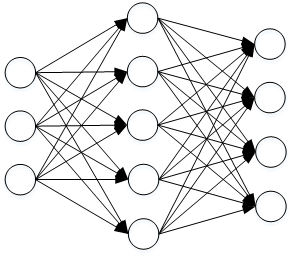
一般的神经网络模型都包括 前向传播 和 反向传播 两个过程。以上图为例：

• 前向传播接收输入 X，然后映射到中间隐藏层 H：
  $H = f(W_1X + b_1)$
  当然，你也可以把每一个隐藏层的行为看成与之前的线性分类器类似，但是需要添加非线性的激活函数 $f()$。
• 然后中间隐藏层 $H$ 再经过映射得到我们的预测分数层 $S$
  $S = f(W_2H+b_2)$
• 这里的 $S$ 我们可以看成之前线性分类器的得分，然后后面使用 $SVM$ 或者 $Softmax$ 进行分类。
• 反向传播阶段就是根据 计算图 和 链式法则 计算出 损失函数对于参数的 梯度，然后用 SGD来更新梯度。
  
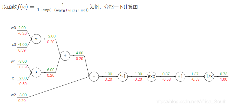
• 上图中，绿色代表前向传播，红色代表反向传播过程。

1. 下载数据集

参照之前的 KNN 分类器

2. 神经网络分类器

• 使用 jupyter nodetebook 打开文件 two_layer_net.ipynb 梳理一下流程（期间没有的python库需要自己手动安装一下）
• 首先，我们需要在cs231n/classifiers/neural_net.py中实现我们的分类器
• 而我们的分类器就类似于上图中的两层神经网络分类器，其网络结果如下
• Input -> Fully Connected Layer -> ReLu -> Fully Connected Layer -> Softmax

2.1 实现神经网络分类器

• 我们实现 neural_net.py\TwoLayerNet中简单分类器的权重初始化、前向传播、反向传播和预测过程。

class TwoLayerNet(object):
  """
  A two-layer fully-connected neural network. 
  The net has an input dimension of N, a hidden layer dimension of H, and performs     classification over C classes.
  
  We train the network with a softmax loss function and L2 regularization on the
  weight matrices. The network uses a ReLU nonlinearity after the first fully
  connected layer.

  The outputs of the second fully-connected layer are the scores for each class.
  """

  def __init__(self, input_size, hidden_size, output_size, std=1e-4):
    """
    Initialize the model. Weights are initialized to small random values and
    biases are initialized to zero. Weights and biases are stored in the
    variable self.params, which is a dictionary with the following keys:

    W1: First layer weights; has shape (D, H)
    b1: First layer biases; has shape (H,)
    W2: Second layer weights; has shape (H, C)
    b2: Second layer biases; has shape (C,)

    Inputs:
    - input_size: The dimension D of the input data.
    - hidden_size: The number of neurons H in the hidden layer.
    - output_size: The number of classes C.
    """
    self.params = {}
    self.params['W1'] = std * np.random.randn(input_size, hidden_size)
    self.params['b1'] = np.zeros(hidden_size)
    self.params['W2'] = std * np.random.randn(hidden_size, output_size)
    self.params['b2'] = np.zeros(output_size)

  def loss(self, X, y=None, reg=0.0):
    """
    Compute the loss and gradients for a two layer fully connected neural
    network.

    Inputs:
    - X: Input data of shape (N, D). Each X[i] is a training sample.
    - y: Vector of training labels. y[i] is the label for X[i], and each y[i] is
      an integer in the range 0 <= y[i] < C. This parameter is optional; if it
      is not passed then we only return scores, and if it is passed then we
      instead return the loss and gradients.
    - reg: Regularization strength.

    Returns:
    If y is None, return a matrix scores of shape (N, C) where scores[i, c] is
    the score for class c on input X[i].

    If y is not None, instead return a tuple of:
    - loss: Loss (data loss and regularization loss) for this batch of training
      samples.
    - grads: Dictionary mapping parameter names to gradients of those parameters
      with respect to the loss function; has the same keys as self.params.
    """
    # Unpack variables from the params dictionary
    W1, b1 = self.params['W1'], self.params['b1']
    W2, b2 = self.params['W2'], self.params['b2']
    N, D = X.shape

    # Compute the forward pass
    scores = None
    h1 = np.dot(X,W1) + b1
    h2 = np.maximum(0,h1) # relu 激活函数
    scores = np.dot(h2,W2) + b2
    # If the targets are not given then jump out, we're done
    if y is None:
      return scores

    # Compute the loss
    loss = None
    # Use the Softmax classifier loss.
    # 得分函数减一个最大值，避免指数结果太大
    scores -= np.max(scores,axis = 1,keepdims = True)
    softmax_output = np.exp(scores) / np.sum(np.exp(scores),axis = 1, keepdims = True)
    loss = np.sum(-np.log(softmax_output[range(N),y])) # 只有正确分类才有损失
    # 添加正则项
    loss /= N# 平均损失
    # 注意：这里我在正则项前面加了一个0.5
    # 所以，可能最后的损失有出入
    loss += 0.5 * reg * np.sum(W1 * W1)
    loss += 0.5 * reg * np.sum(W2 * W2)
    # Backward pass: compute gradients
    grads = {}
    # Store the results in the grads dictionary. For example,       #
    # grads['W1'] should store the gradient on W1, and be a matrix of same size #
    dS = softmax_output.copy()
    # 正确分类项要减1
    dS[range(h2.shape[0]),y] -= 1 # 对得分矩阵的梯度矩阵
    # 注意，这里的损失应该是N个样本的平均损失
    dS /= N
    # 然后是 h2 * W2 + b2 = S
    grads["W2"] = np.dot(h2.T,dS)
    dh2 = np.dot(dS,W2.T)
    grads["b2"] = np.sum(dS,axis = 0) # 这里已经取过平均值了
    # 然后是 h2 = relu(h1)
    dh1 = dh2
    dh1[h1 <= 0] = 0
    # 最后是 h1 = X * W1 + b1
    grads["W1"] = np.dot(X.T,dh1)
    grads["b1"] = np.sum(dh1,axis = 0)
    # 加上正则项
    grads["W1"] += reg * W1
    grads["W2"] += reg * W2
    return loss, grads

  def train(self, X, y, X_val, y_val,
            learning_rate=1e-3, learning_rate_decay=0.95,
            reg=5e-6, num_iters=100,
            batch_size=200, verbose=False):
    """
    Train this neural network using stochastic gradient descent.

    Inputs:
    - X: A numpy array of shape (N, D) giving training data.
    - y: A numpy array f shape (N,) giving training labels; y[i] = c means that
      X[i] has label c, where 0 <= c < C.
    - X_val: A numpy array of shape (N_val, D) giving validation data.
    - y_val: A numpy array of shape (N_val,) giving validation labels.
    - learning_rate: Scalar giving learning rate for optimization.
    - learning_rate_decay: Scalar giving factor used to decay the learning rate
      after each epoch.
    - reg: Scalar giving regularization strength.
    - num_iters: Number of steps to take when optimizing.
    - batch_size: Number of training examples to use per step.
    - verbose: boolean; if true print progress during optimization.
    """
    num_train = X.shape[0]
    iterations_per_epoch = max(num_train / batch_size, 1) # 训练全部样本一轮需要的迭代次数

    # Use SGD to optimize the parameters in self.model
    loss_history = []
    train_acc_history = []
    val_acc_history = []

    for it in range(num_iters):
      # TODO: Create a random minibatch of training data and labels, storing  #
      # them in X_batch and y_batch respectively.                             #
      # 样本的起始点
      idx_batch = np.random.choice(num_train,batch_size,replace = True)
      X_batch = X[idx_batch]
      y_batch = y[idx_batch]

      # Compute loss and gradients using the current minibatch
      loss, grads = self.loss(X_batch, y=y_batch, reg=reg)
      loss_history.append(loss)
      self.params['W1'] += -learning_rate * grads['W1']
      self.params['b1'] += -learning_rate * grads['b1']
      self.params['W2'] += -learning_rate * grads['W2']
      self.params['b2'] += -learning_rate * grads['b2']

      if verbose and it % 100 == 0:
        print('iteration %d / %d: loss %f' % (it, num_iters, loss))

      # Every epoch, check train and val accuracy and decay learning rate.
      if it % iterations_per_epoch == 0:
        # Check accuracy
        train_acc = (self.predict(X_batch) == y_batch).mean()
        val_acc = (self.predict(X_val) == y_val).mean()
        train_acc_history.append(train_acc)
        val_acc_history.append(val_acc)

        # Decay learning rate
        learning_rate *= learning_rate_decay

    return {
      'loss_history': loss_history,
      'train_acc_history': train_acc_history,
      'val_acc_history': val_acc_history,
    }

  def predict(self, X):
    """
    Use the trained weights of this two-layer network to predict labels for
    data points. For each data point we predict scores for each of the C
    classes, and assign each data point to the class with the highest score.

    Inputs:
    - X: A numpy array of shape (N, D) giving N D-dimensional data points to
      classify.

    Returns:
    - y_pred: A numpy array of shape (N,) giving predicted labels for each of
      the elements of X. For all i, y_pred[i] = c means that X[i] is predicted
      to have class c, where 0 <= c < C.
    """
    W1 = self.params['W1']
    b1 = self.params['b1']
    W2 = self.params['W2']
    b2 = self.params['b2']
    h1 = np.dot(X,W1) + b1
    h2 = np.maximum(0,h1)
    scores = np.dot(h2,W2) + b2
    y_pred = np.argmax(scores,axis = 1)
    return y_pred

2.2 测试实现正确性

创建一个测试数据来验证我们实现的损失和得分函数的正确性

import numpy as np
import matplotlib.pyplot as plt

from cs231n.classifiers.neural_net import TwoLayerNet

from __future__ import print_function

%matplotlib inline
plt.rcParams['figure.figsize'] = (10.0, 8.0) # set default size of plots
plt.rcParams['image.interpolation'] = 'nearest'
plt.rcParams['image.cmap'] = 'gray'

# for auto-reloading external modules
# see http://stackoverflow.com/questions/1907993/autoreload-of-modules-in-ipython
%load_ext autoreload
%autoreload 2

def rel_error(x, y):
    """ returns relative error """
    return np.max(np.abs(x - y) / (np.maximum(1e-8, np.abs(x) + np.abs(y))))

# Create a small net and some toy data to check your implementations.
# Note that we set the random seed for repeatable experiments.

input_size = 4
hidden_size = 10
num_classes = 3
num_inputs = 5

def init_toy_model():
    np.random.seed(0)
    return TwoLayerNet(input_size, hidden_size, num_classes, std=1e-1)

def init_toy_data():
    np.random.seed(1)
    X = 10 * np.random.randn(num_inputs, input_size)
    y = np.array([0, 1, 2, 2, 1])
    return X, y

net = init_toy_model()
X, y = init_toy_data()

验证得分函数

• 对应于TwoLayerNet.loss()方法，只要不输入Y，则返回其得分

scores = net.loss(X)
print('Your scores:')
print(scores)
print()
print('correct scores:')
correct_scores = np.asarray([
  [-0.81233741, -1.27654624, -0.70335995],
  [-0.17129677, -1.18803311, -0.47310444],
  [-0.51590475, -1.01354314, -0.8504215 ],
  [-0.15419291, -0.48629638, -0.52901952],
  [-0.00618733, -0.12435261, -0.15226949]])
print(correct_scores)
print()

# The difference should be very small. We get < 1e-7
print('Difference between your scores and correct scores:')
print(np.sum(np.abs(scores - correct_scores)))

由于我们的随机数种子固定，所以我们每次实验产生的随机数相同，所以会有标准答案。

验证损失函数

• 对应于TwoLayerNet.loss()方法，需要输入标签y

loss, _ = net.loss(X, y, reg=0.05)
print("your loss is {}".format(loss))
correct_loss = 1.30378789133

# should be very small, we get < 1e-12
print('Difference between your loss and correct loss:')
print(np.sum(np.abs(loss - correct_loss)))

注意：由于我个人在损失函数的L2正则项前添加了一个系数0.5，所以可能最后计算出来的损失和官方有一定的出入。

your loss is 1.28482247172
Difference between your loss and correct loss:
0.0189654196061

梯度检验
对应于TwoLayerNet.loss()方法,返回损失+梯度字典

from cs231n.gradient_check import eval_numerical_gradient

# Use numeric gradient checking to check your implementation of the backward pass.
# If your implementation is correct, the difference between the numeric and
# analytic gradients should be less than 1e-8 for each of W1, W2, b1, and b2.

loss, grads = net.loss(X, y, reg=0.05)

# these should all be less than 1e-8 or so
for param_name in grads:
    f = lambda W: net.loss(X, y, reg=0.05)[0]
    param_grad_num = eval_numerical_gradient(f, net.params[param_name], verbose=False)
    print('%s max relative error: %e' % (param_name, rel_error(param_grad_num, grads[param_name])))

训练网络

• 对应于TwoLayerNet.train()方法，返回损失历史、训练集精度、验证集精度的一个字典

net = init_toy_model()
stats = net.train(X, y, X, y,
            learning_rate=1e-1, reg=5e-6,
            num_iters=100, verbose=False)

print('Final training loss: ', stats['loss_history'][-1])

# plot the loss history
plt.plot(stats['loss_history'])
plt.xlabel('iteration')
plt.ylabel('training loss')
plt.title('Training Loss history')
plt.show()

2.3 在真实数据集CIFAR10上测试

加载并划分数据集

from cs231n.data_utils import load_CIFAR10

def get_CIFAR10_data(num_training=49000, num_validation=1000, num_test=1000):
    """
    Load the CIFAR-10 dataset from disk and perform preprocessing to prepare
    it for the two-layer neural net classifier. These are the same steps as
    we used for the SVM, but condensed to a single function.  
    """
    # Load the raw CIFAR-10 data
    cifar10_dir = 'cs231n/datasets/cifar-10-batches-py'
    
    X_train, y_train, X_test, y_test = load_CIFAR10(cifar10_dir)
        
    # Subsample the data
    mask = list(range(num_training, num_training + num_validation))
    X_val = X_train[mask]
    y_val = y_train[mask]
    mask = list(range(num_training))
    X_train = X_train[mask]
    y_train = y_train[mask]
    mask = list(range(num_test))
    X_test = X_test[mask]
    y_test = y_test[mask]

    # Normalize the data: subtract the mean image
    mean_image = np.mean(X_train, axis=0)
    X_train -= mean_image
    X_val -= mean_image
    X_test -= mean_image

    # Reshape data to rows
    X_train = X_train.reshape(num_training, -1)
    X_val = X_val.reshape(num_validation, -1)
    X_test = X_test.reshape(num_test, -1)

    return X_train, y_train, X_val, y_val, X_test, y_test


# Cleaning up variables to prevent loading data multiple times (which may cause memory issue)
try:
   del X_train, y_train
   del X_test, y_test
   print('Clear previously loaded data.')
except:
   pass

# Invoke the above function to get our data.
X_train, y_train, X_val, y_val, X_test, y_test = get_CIFAR10_data()
print('Train data shape: ', X_train.shape)
print('Train labels shape: ', y_train.shape)
print('Validation data shape: ', X_val.shape)
print('Validation labels shape: ', y_val.shape)
print('Test data shape: ', X_test.shape)
print('Test labels shape: ', y_test.shape)

训练神经网络

• 每一次batch迭代都产生一个训练损失；
• 每次进行整个训练集迭代(epoch)产生一个训练精度和验证精度。

input_size = 32 * 32 * 3
hidden_size = 50
num_classes = 10
net = TwoLayerNet(input_size, hidden_size, num_classes)

# Train the network
stats = net.train(X_train, y_train, X_val, y_val,
            num_iters=1000, batch_size=200,
            learning_rate=1e-4, learning_rate_decay=0.95,
            reg=0.25, verbose=True)

# Predict on the validation set
val_acc = (net.predict(X_val) == y_val).mean()
print('Validation accuracy: ', val_acc)

iteration 0 / 1000: loss 2.302781
iteration 100 / 1000: loss 2.302350
iteration 200 / 1000: loss 2.298087
iteration 300 / 1000: loss 2.254848
iteration 400 / 1000: loss 2.181098
iteration 500 / 1000: loss 2.129994
iteration 600 / 1000: loss 2.124660
iteration 700 / 1000: loss 2.061074
iteration 800 / 1000: loss 2.037901
iteration 900 / 1000: loss 1.987142
Validation accuracy:  0.277

调试训练过程
可以看到，我们初步得到的验证集的精度只有0.277，所以我们可以画训练过程中的损失函数变化，和训练集和验证集的准确度变化过程，来看我们的训练进行的怎么样了。

plt.subplot(2, 1, 1)
plt.plot(stats['loss_history'])
plt.title('Loss history')
plt.xlabel('Iteration')
plt.ylabel('Loss')

plt.subplot(2, 1, 2)
plt.plot(stats['train_acc_history'], label='train')
plt.plot(stats['val_acc_history'], label='val')
plt.title('Classification accuracy history')
plt.xlabel('Epoch')
plt.ylabel('Clasification accuracy')
plt.legend()
plt.show()

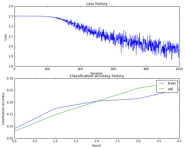
可以看到，我们起始就在整个数据集上迭代了4个epoch，或许损失和精度都还没有达到收敛状态。

可视化第一层的权重
我们的输入是 $[N,D]$，而我们第一层的权重是 $[D,H]$，根据之前线性分类器的知识，我们其实可以将其看成 H 个模板来看待，所以，可以用之前的方法可视化第一层的权重。

from cs231n.vis_utils import visualize_grid

# Visualize the weights of the network

def show_net_weights(net):
    W1 = net.params['W1']
    W1 = W1.reshape(32, 32, 3, -1).transpose(3, 0, 1, 2)
    plt.imshow(visualize_grid(W1, padding=3).astype('uint8'))
    plt.gca().axis('off')
    plt.show()

show_net_weights(net)

而方格显示函数visualize_grid()也就是把可我们的50个权重复制到一个大方格中。

def visualize_grid(Xs, ubound=255.0, padding=1):
  """
  Reshape a 4D tensor of image data to a grid for easy visualization.

  Inputs:
  - Xs: Data of shape (N, H, W, C)
  - ubound: Output grid will have values scaled to the range [0, ubound]
  - padding: The number of blank pixels between elements of the grid
  """
  (N, H, W, C) = Xs.shape
  grid_size = int(ceil(sqrt(N)))
  grid_height = H * grid_size + padding * (grid_size - 1)
  grid_width = W * grid_size + padding * (grid_size - 1)
  grid = np.zeros((grid_height, grid_width, C))
  next_idx = 0
  y0, y1 = 0, H
  for y in range(grid_size):
    x0, x1 = 0, W
    for x in range(grid_size):
      if next_idx < N:
        img = Xs[next_idx]
        low, high = np.min(img), np.max(img)
        grid[y0:y1, x0:x1] = ubound * (img - low) / (high - low)
        # grid[y0:y1, x0:x1] = Xs[next_idx]
        next_idx += 1
      x0 += W + padding
      x1 += W + padding
    y0 += H + padding
    y1 += H + padding
  # grid_max = np.max(grid)
  # grid_min = np.min(grid)
  # grid = ubound * (grid - grid_min) / (grid_max - grid_min)
  return grid

从上图中可以看到，里面有些模板有点像我们之前的汽车模板。

2.5 调节参数

• 调节我们的超参数：学习率，惩罚强度，中间隐藏层结点等超参数。

# 网络结构
input_size = 32 * 32 * 3
num_classes = 10

# 超级参数
hidden_num = [40,80,160]
learning_rate_choice = [1e-4, 5e-4, 9e-4, 13e-4, 15e-4]
reg_choice = [5e-6,5e-5,5e-4]
num_iters = 3000
batch_size = 256
learning_rate_decay = 0.98

# 中间结果
best_net = None
best_hidden = None
best_lr = None
best_reg = None
best_val = -1 # 最好的验证集精度
results = {} # 存储训练集和验证集的精度

for hidden in hidden_num:
    for lr in learning_rate_choice:
        for reg in reg_choice:
            net = TwoLayerNet(input_size,hidden,num_classes)
            stats = net.train(X=X_train,y=y_train,X_val = X_val,y_val=y_val,
                              learning_rate=lr,reg=reg,num_iters=num_iters,batch_size = batch_size)
            results[(hidden,lr,reg)] = (stats["train_acc_history"][-1],stats["val_acc_history"][-1])
            # 当然，我认为更好的方式可能是每个 epoch 之后都检查以下精度是否提升
            train_acc = stats["train_acc_history"][-1] # 有多个epoch
            val_acc = stats["val_acc_history"][-1] # 有多个epoch
            if val_acc > best_val:
                best_val = val_acc
                best_lr = lr
                best_reg = reg
                best_hidden = hidden
                best_net = net
            print("hidden_size:%d lr:%e reg:%e train_acc:%f val_acc:%f" %
                 (hidden,lr,reg,train_acc,val_acc))
            
print('Best hidden_size: %d\n Best lr: %e\nBest reg: %e\ntrain accuracy: %f\nval accuracy: %f' %
     (best_hidden, best_lr, best_reg, results[(best_hidden,best_lr, best_reg)][0], results[(best_hidden,best_lr, best_reg)][1]))

Best hidden_size: 160
Best lr: 9.000000e-04
Best reg: 5.000000e-04
train accuracy: 0.660156
val accuracy: 0.541000

可视化交叉验证结果

• 像之前的实验一样，对于每个中间隐藏层参数，画出其（学习率，惩罚强度）对应的准确度。
• 白色区域表示精度大

# Visualize the cross-validation results
import math

marker_size = 100
for i,hidden in enumerate(hidden_num):
        x_scatter = [math.log10(x[1]) for x in results if x[0] == hidden] # 学习率
        y_scatter = [math.log10(x[2]) for x in results if x[0] == hidden] # 惩罚强度
        # 画训练集
        colors = [results[x][0] for x in results if x[0] == hidden]
        plt.subplot(3,2,2*i+1)
        plt.scatter(x_scatter,y_scatter,marker_size,c=colors)
        plt.colorbar()
        plt.xlabel('log learning rate')
        plt.ylabel('log regularization strength')
        plt.title('hidden_num = %d training accuracy' % hidden)
        # 画测试集
        colors = [results[x][1] for x in results if x[0] == hidden]
        plt.subplot(3,2,2*i+2)
        plt.scatter(x_scatter,y_scatter,marker_size,c=colors)
        plt.colorbar()
        plt.xlabel('log learning rate')
        plt.ylabel('log regularization strength')
        plt.title('hidden_num = %d validation accuracy' % hidden)
plt.subplots_adjust(hspace = 0.6)
plt.show()

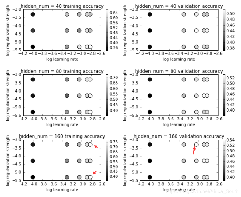
• 由上图可知，低学习率的模型最后的精度普遍小，可能的原因是模拟并未收敛，需要增加迭代次数。

可视化第一层权重

from vis_utils import visualize_grid

# Visualize the weights of the network
def show_net_weights(net):
    W1 = net.params['W1']
    W1 = W1.reshape(32, 32, 3, -1).transpose(3, 0, 1, 2)
    plt.imshow(visualize_grid(W1, padding=3).astype('uint8'))
    plt.gca().axis('off')
    plt.show()

show_net_weights(net)

• 可以发现，相比于之前的50个模板，这里的160个模板更加丰富而且由于迭代次数的增加，表现得也更加得magic。

2.6 测试集(test)上测试

test_acc = (best_net.predict(X_test) == y_test).mean()
print('Test accuracy: ', test_acc)
# Test accuracy:  0.529

作业问题

• Q1: Now that you have trained a Neural Network classifier, you may find that your testing accuracy is much lower than the training accuracy. In what ways can we decrease this gap? Select all that apply.

  1.Train on a larger dataset.
  2.Add more hidden units.
  3.Increase the regularization strength.
  4.None of the above.

• A1: 可选的操作：在更大的训练集上训练，增加正则强度。增加更多的隐藏层结点可能没有效果，因为增加了模拟的复杂度，使其更加的拟合训练集，从而进一步的加大了训练集和测试集的性能差异。

参考资料

• cs231n linear classification notes
• cs231n Optimization: Stochastic Gradient Descent
• cs231n Backpropagation, Intuitions