【cs231n】assignment1 ：k-Nearest Neighbor classifier

记录cs231n课程的课后作业。这里主要是assignment1里的k-Nearest Neighbor classifier。代码参考来自这里。
运行平台：win7+64位+jupyter notebook

1 搭建运行平台

根据作业的官方网站介绍，这个作业使用的是python语言，可以采用Google Cloud和Workinglocally这两种方法来做作业，这里只能选择后者。所以第一步要安装好python以及jupyter notebook。接着下载作业代码以及CIFAR-10数据库，官方是使用get_datasets.sh文件来下载这个数据库的，在windows平台上就直接手动下载好并解压放在对应的文件夹中，至此完成前期的准备工作。文件夹里的各文件如下所示：

文件示意图

2 运行knn.ipynb文件

k-Nearest Neighbor classifier所对应的运行文件就是knn.ipynb文件。这里的文件分为好多个cell，按顺序运行每个cell，有的cell会调用到cs231n.classifiers里面的KNearestNeighbor函数，其中有部分代码需要自己编写完整。

k-Nearest Neighbor (kNN) exercise
Complete and hand in this completed worksheet (including its outputs and any supporting code outside of the worksheet) with your assignment submission. For more details see the assignments page on the course website.
The kNN classifier consists of two stages:
During training, the classifier takes the training data and simply remembers it
During testing, kNN classifies every test image by comparing to all training images and transfering the labels of the k most similar training examples
The value of k is cross-validated
In this exercise you will implement these steps and understand the basic Image Classification pipeline, cross-validation, and gain proficiency in writing efficient, vectorized code.

根据这段官方的介绍，我们了解到接下来要训练一个KNN（K近邻）分类器，分为训练过程和测试过程，并将采用交叉验证的方式来确定k的值。

setup步骤和运行结果。

# Run some setup code for this notebook.

import random
import numpy as np
from cs231n.data_utils import load_CIFAR10
import matplotlib.pyplot as plt

from __future__ import print_function

# This is a bit of magic to make matplotlib figures appear inline in the notebook
# rather than in a new window.
%matplotlib inline
plt.rcParams['figure.figsize'] = (10.0, 8.0) # set default size of plots
plt.rcParams['image.interpolation'] = 'nearest'
plt.rcParams['image.cmap'] = 'gray'

# Some more magic so that the notebook will reload external python modules;
# see http://stackoverflow.com/questions/1907993/autoreload-of-modules-in-ipython
%load_ext autoreload
%autoreload 2

The autoreload extension is already loaded. To reload it, use:
  %reload_ext autoreload

加载CIFAR-10数据。

cifar10_dir = 'cs231n/datasets/cifar-10-batches-py'
X_train, y_train, X_test, y_test = load_CIFAR10(cifar10_dir)

# As a sanity check, we print out the size of the training and test data.
print('Training data shape: ', X_train.shape)
print('Training labels shape: ', y_train.shape)
print('Test data shape: ', X_test.shape)
print('Test labels shape: ', y_test.shape)

Training data shape:  (50000, 32, 32, 3)
Training labels shape:  (50000,)
Test data shape:  (10000, 32, 32, 3)
Test labels shape:  (10000,)

可视化某些数据，可以看出这些图像尺寸都是32*32*3，每个图像都有一个对应的label。

# Visualize some examples from the dataset.
# We show a few examples of training images from each class.
classes = ['plane', 'car', 'bird', 'cat', 'deer', 'dog', 'frog', 'horse', 'ship', 'truck']
num_classes = len(classes)
samples_per_class = 7
for y, cls in enumerate(classes):
    idxs = np.flatnonzero(y_train == y)
    idxs = np.random.choice(idxs, samples_per_class, replace=False)
    for i, idx in enumerate(idxs):
        plt_idx = i * num_classes + y + 1
        plt.subplot(samples_per_class, num_classes, plt_idx)
        plt.imshow(X_train[idx].astype('uint8'))
        plt.axis('off')
        if i == 0:
            plt.title(cls)
plt.show()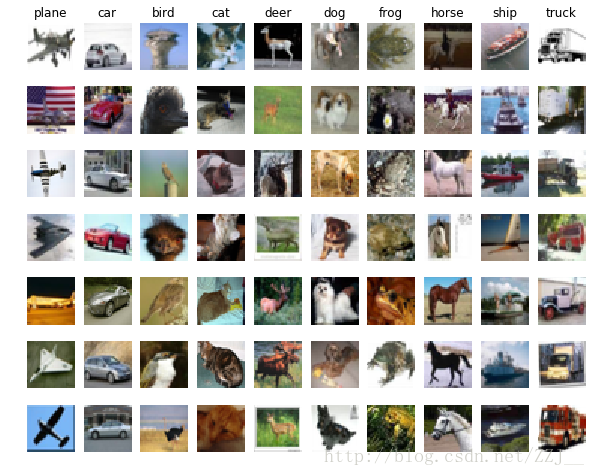

可视化结果

选取5000个训练数据和500个测试数据。

# Subsample the data for more efficient code execution in this exercise
num_training = 5000
mask = list(range(num_training))
X_train = X_train[mask]
y_train = y_train[mask]

num_test = 500
mask = list(range(num_test))
X_test = X_test[mask]
y_test = y_test[mask]

将这些图像数据向量化（32*32*3=3072）。

# Reshape the image data into rows
X_train = np.reshape(X_train, (X_train.shape[0], -1))
X_test = np.reshape(X_test, (X_test.shape[0], -1))
print(X_train.shape, X_test.shape)
print(y_train.shape, y_test.shape)

(5000, 3072) (500, 3072)
(5000,) (500,)

调用KNearestNeighbor进行训练。

from cs231n.classifiers import KNearestNeighbor

# Create a kNN classifier instance. 
# Remember that training a kNN classifier is a noop: 
# the Classifier simply remembers the data and does no further processing 
classifier = KNearestNeighbor()
classifier.train(X_train, y_train)

计算测试数据和训练数据之间的距离。计算所有的test examples和所有的train examples之间的距离，对于每个给定的test example，我们都能够找到离它最近的k个train examples，从而投票得出这个test example的label。下面结果表示计算的距离结果存放在500*5000的数据结构中。

# Open cs231n/classifiers/k_nearest_neighbor.py and implement
# compute_distances_two_loops.

# Test your implementation:
dists = classifier.compute_distances_two_loops(X_test)
print(dists.shape)

(500, 5000)

将计算的距离可视化。

# We can visualize the distance matrix: each row is a single test example and
# its distances to training examples
plt.imshow(dists, interpolation='none')
plt.show()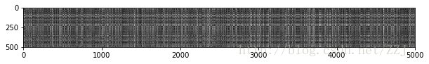

距离结果可视化

Inline Question #1:
Question：What in the data is the cause behind the distinctly bright rows?What causes the columns?
Answer:
取k为1，测试此时的模型预测正确率

# Now implement the function predict_labels and run the code below:
# We use k = 1 (which is Nearest Neighbor).
y_test_pred = classifier.predict_labels(dists, k=1)

# Compute and print the fraction of correctly predicted examples
num_correct = np.sum(y_test_pred == y_test)
accuracy = float(num_correct) / num_test
print('Got %d / %d correct => accuracy: %f' % (num_correct, num_test, accuracy))

Got 137 / 500 correct => accuracy: 0.274000

将k取值改为5，再测试此时的预测准确率（比k为1时稍微好一点）。

y_test_pred = classifier.predict_labels(dists, k=5)
num_correct = np.sum(y_test_pred == y_test)
accuracy = float(num_correct) / num_test
print('Got %d / %d correct => accuracy: %f' % (num_correct, num_test, accuracy))

Got 139 / 500 correct => accuracy: 0.278000

采用one-loop的方式来计算距离，并与之前的dists进行比较。

# Now lets speed up distance matrix computation by using partial vectorization
# with one loop. Implement the function compute_distances_one_loop and run the
# code below:
dists_one = classifier.compute_distances_one_loop(X_test)

# To ensure that our vectorized implementation is correct, we make sure that it
# agrees with the naive implementation. There are many ways to decide whether
# two matrices are similar; one of the simplest is the Frobenius norm. In case
# you haven't seen it before, the Frobenius norm of two matrices is the square
# root of the squared sum of differences of all elements; in other words, reshape
# the matrices into vectors and compute the Euclidean distance between them.
difference = np.linalg.norm(dists - dists_one, ord='fro')
print('Difference was: %f' % (difference, ))
if difference < 0.001:
    print('Good! The distance matrices are the same')
else:
    print('Uh-oh! The distance matrices are different')

Difference was: 0.000000
Good! The distance matrices are the same

采用完全向量化的计算方式来计算距离，并与dists进行比较。

# Now implement the fully vectorized version inside compute_distances_no_loops
# and run the code
dists_two = classifier.compute_distances_no_loops(X_test)

# check that the distance matrix agrees with the one we computed before:
difference = np.linalg.norm(dists - dists_two, ord='fro')
print('Difference was: %f' % (difference, ))
if difference < 0.001:
    print('Good! The distance matrices are the same')
else:
    print('Uh-oh! The distance matrices are different')

Difference was: 0.000000
Good! The distance matrices are the same

比较以上几种计算方法的耗时。

# Let's compare how fast the implementations are
def time_function(f, *args):
    """
    Call a function f with args and return the time (in seconds) that it took to execute.
    """
    import time
    tic = time.time()
    f(*args)
    toc = time.time()
    return toc - tic

two_loop_time = time_function(classifier.compute_distances_two_loops, X_test)
print('Two loop version took %f seconds' % two_loop_time)

one_loop_time = time_function(classifier.compute_distances_one_loop, X_test)
print('One loop version took %f seconds' % one_loop_time)

no_loop_time = time_function(classifier.compute_distances_no_loops, X_test)
print('No loop version took %f seconds' % no_loop_time)

# you should see significantly faster performance with the fully vectorized implementation

Two loop version took 33.328906 seconds
One loop version took 64.720702 seconds
No loop version took 0.329019 seconds

Cross-validation 交叉验证

num_folds = 5
k_choices = [1, 3, 5, 8, 10, 12, 15, 20, 50, 100]

X_train_folds = []
y_train_folds = []
################################################################################
# TODO:                                                                        #
# Split up the training data into folds. After splitting, X_train_folds and    #
# y_train_folds should each be lists of length num_folds, where                #
# y_train_folds[i] is the label vector for the points in X_train_folds[i].     #
# Hint: Look up the numpy array_split function.                                #
################################################################################
y_train_ = y_train.reshape(-1, 1)
X_train_folds , y_train_folds = np.array_split(X_train, 5), np.array_split(y_train_, 5)
################################################################################
#                                 END OF YOUR CODE                             #
################################################################################

# A dictionary holding the accuracies for different values of k that we find
# when running cross-validation. After running cross-validation,
# k_to_accuracies[k] should be a list of length num_folds giving the different
# accuracy values that we found when using that value of k.
k_to_accuracies = {}


################################################################################
# TODO:                                                                        #
# Perform k-fold cross validation to find the best value of k. For each        #
# possible value of k, run the k-nearest-neighbor algorithm num_folds times,   #
# where in each case you use all but one of the folds as training data and the #
# last fold as a validation set. Store the accuracies for all fold and all     #
# values of k in the k_to_accuracies dictionary.                               #
################################################################################
for k_ in k_choices:
    k_to_accuracies.setdefault(k_, [])
for i in range(num_folds):
    classifier = KNearestNeighbor()
    X_val_train = np.vstack(X_train_folds[0:i] + X_train_folds[i+1:])
    y_val_train = np.vstack(y_train_folds[0:i] + y_train_folds[i+1:])
    y_val_train = y_val_train[:,0]
    classifier.train(X_val_train, y_val_train)
    for k_ in k_choices:
        y_val_pred = classifier.predict(X_train_folds[i], k=k_)
        num_correct = np.sum(y_val_pred == y_train_folds[i][:,0])
        accuracy = float(num_correct) / len(y_val_pred)
        k_to_accuracies[k_] = k_to_accuracies[k_] + [accuracy]
################################################################################
#                                 END OF YOUR CODE                             #
################################################################################

# Print out the computed accuracies
for k in sorted(k_to_accuracies):
    for accuracy in k_to_accuracies[k]:
        print('k = %d, accuracy = %f' % (k, accuracy))

k = 1, accuracy = 0.263000
k = 1, accuracy = 0.257000
k = 1, accuracy = 0.264000
k = 1, accuracy = 0.278000
k = 1, accuracy = 0.266000
k = 3, accuracy = 0.239000
k = 3, accuracy = 0.249000
k = 3, accuracy = 0.240000
k = 3, accuracy = 0.266000
k = 3, accuracy = 0.254000
k = 5, accuracy = 0.248000
k = 5, accuracy = 0.266000
k = 5, accuracy = 0.280000
k = 5, accuracy = 0.292000
k = 5, accuracy = 0.280000
k = 8, accuracy = 0.262000
k = 8, accuracy = 0.282000
k = 8, accuracy = 0.273000
k = 8, accuracy = 0.290000
k = 8, accuracy = 0.273000
k = 10, accuracy = 0.265000
k = 10, accuracy = 0.296000
k = 10, accuracy = 0.276000
k = 10, accuracy = 0.284000
k = 10, accuracy = 0.280000
k = 12, accuracy = 0.260000
k = 12, accuracy = 0.295000
k = 12, accuracy = 0.279000
k = 12, accuracy = 0.283000
k = 12, accuracy = 0.280000
k = 15, accuracy = 0.252000
k = 15, accuracy = 0.289000
k = 15, accuracy = 0.278000
k = 15, accuracy = 0.282000
k = 15, accuracy = 0.274000
k = 20, accuracy = 0.270000
k = 20, accuracy = 0.279000
k = 20, accuracy = 0.279000
k = 20, accuracy = 0.282000
k = 20, accuracy = 0.285000
k = 50, accuracy = 0.271000
k = 50, accuracy = 0.288000
k = 50, accuracy = 0.278000
k = 50, accuracy = 0.269000
k = 50, accuracy = 0.266000
k = 100, accuracy = 0.256000
k = 100, accuracy = 0.270000
k = 100, accuracy = 0.263000
k = 100, accuracy = 0.256000
k = 100, accuracy = 0.263000

画图

# plot the raw observations
for k in k_choices:
    accuracies = k_to_accuracies[k]
    plt.scatter([k] * len(accuracies), accuracies)

# plot the trend line with error bars that correspond to standard deviation
accuracies_mean = np.array([np.mean(v) for k,v in sorted(k_to_accuracies.items())])
accuracies_std = np.array([np.std(v) for k,v in sorted(k_to_accuracies.items())])
plt.errorbar(k_choices, accuracies_mean, yerr=accuracies_std)
plt.title('Cross-validation on k')
plt.xlabel('k')
plt.ylabel('Cross-validation accuracy')
plt.show()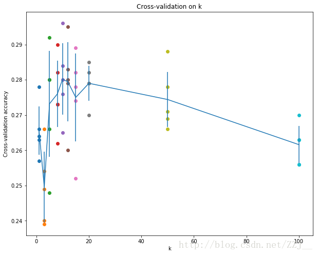

这里写图片描述

根据交叉验证结果，选择最佳的k值。

# Based on the cross-validation results above, choose the best value for k,   
# retrain the classifier using all the training data, and test it on the test
# data. You should be able to get above 28% accuracy on the test data.
best_k = 10

classifier = KNearestNeighbor()
classifier.train(X_train, y_train)
y_test_pred = classifier.predict(X_test, k=best_k)

# Compute and display the accuracy
num_correct = np.sum(y_test_pred == y_test)
accuracy = float(num_correct) / num_test
print 'Got %d / %d correct => accuracy: %f' % (num_correct, num_test, accuracy)

Got 141 / 500 correct => accuracy: 0.282000