Programming Exercise 2: Logistic Regression
Python版本3.6
编译环境:anaconda Jupyter Notebook
链接:ex2data1.txt、ex2data2.txt 和编程作业ex2.pdf(实验指导书)
提取码:i7co
本章课程笔记部分见:逻辑回归 正则化
在这一次练习中,我们将要实现逻辑回归并且应用到一个分类任务。我们还将通过将正则化加入训练算法,来提高算法的鲁棒性,并用更复杂的情形来测试它。
样本训练数据为申请入学的学生两次测评的成绩,以及最后是否被录取的结果。
%matplotlib inline
#IPython的内置magic函数,可以省掉plt.show(),在其他IDE中是不会支持的
import numpy as np
import pandas as pd
import matplotlib as mpl
import matplotlib.pyplot as plt
import seaborn as sns
sns.set(style="whitegrid",color_codes=True)
data = pd.read_csv('ex2data1.txt', header=None, names=['Exam 1', 'Exam 2', 'Admitted'])
data.head()
| Exam 1 | Exam 2 | Admitted | |
|---|---|---|---|
| 0 | 34.623660 | 78.024693 | 0 |
| 1 | 30.286711 | 43.894998 | 0 |
| 2 | 35.847409 | 72.902198 | 0 |
| 3 | 60.182599 | 86.308552 | 1 |
| 4 | 79.032736 | 75.344376 | 1 |
数据可视化
创建两个分数的散点图,并使用颜色编码来可视化,如果样本是正的(被接纳)或负的(未被接纳)。
positive = data[data['Admitted'].isin([1])]
negative = data[data['Admitted'].isin([0])]

fig, ax = plt.subplots(figsize=(10,6))
ax.scatter(positive['Exam 1'], positive['Exam 2'], s=50, c='b', marker='o', label='Admitted')
ax.scatter(negative['Exam 1'], negative['Exam 2'], s=50, c='r', marker='x', label='Not Admitted')
ax.legend()
ax.set_xlabel('Exam 1 Score')
ax.set_ylabel('Exam 2 Score')
Text(0, 0.5, 'Exam 2 Score')

看起来在两类间,有一个清晰的决策边界。现在我们需要实现逻辑回归,那样就可以训练一个分类模型来预测结果。
sigmoid 函数
g 代表一个常用的逻辑函数(logistic function)为S形函数(Sigmoid function),公式为: \[g\left( z \right)=\frac{1}{1+{{e}^{-z}}}\]
合起来,我们得到逻辑回归模型的假设函数:
\[{{h}_{\theta }}\left( x \right)=\frac{1}{1+{{e}^{-{{\theta }^{T}}X}}}\]
def sigmoid(z):
    return 1 / (1 + np.exp(-z))
nums = np.arange(-10, 10, step=0.01)

fig, ax = plt.subplots(figsize=(8,6))
ax.plot(nums, sigmoid(nums), 'r')
[<matplotlib.lines.Line2D at 0x93d7c31710>]

代价函数:
def cost(theta, X, y):
    theta = np.matrix(theta)
    X = np.matrix(X)
    y = np.matrix(y)
    first = np.multiply(-y, np.log(sigmoid(X * theta.T)))
    second = np.multiply((1 - y), np.log(1 - sigmoid(X * theta.T)))
    return np.sum(first - second) / (len(X))
对数据稍作处理,同exercise1
# add a ones column - this makes the matrix multiplication work out easier
data.insert(0, 'Ones', 1)

# set X (training data) and y (target variable)
cols = data.shape[1]
X = data.iloc[:,0:cols-1]
y = data.iloc[:,cols-1:cols]

# convert to numpy arrays and initalize the parameter array theta
X = np.array(X.values)
y = np.array(y.values)
theta = np.zeros(3)
#计算一下初始化参数的cost
cost(theta, X, y)
0.6931471805599453
gradient descent(梯度下降)
- 这是批量梯度下降(batch gradient descent)
- 转化为向量化计算:
#计算一个梯度步长
def gradient(theta, X, y):
    theta = np.matrix(theta)
    X = np.matrix(X)
    y = np.matrix(y)

    parameters = int(theta.ravel().shape[1])
    grad = np.zeros(parameters)

    error = sigmoid(X * theta.T) - y

    for i in range(parameters):
        term = np.multiply(error, X[:,i])
        grad[i] = np.sum(term) / len(X)

    return grad
使用 scipy.optimize.minimize 去拟合参数
import scipy.optimize as opt
res = opt.minimize(fun=cost, x0=theta, args=(X, y), method='Newton-CG', jac=gradient)
res
     fun: 0.2034977018633035
     jac: array([-2.12380382e-05, -1.40885753e-03, -1.27811598e-03])
 message: 'Optimization terminated successfully.'
    nfev: 72
    nhev: 0
     nit: 28
    njev: 241
  status: 0
 success: True
       x: array([-25.16007951,   0.20622062,   0.20146256])
预测与验证
接下来,我们需要编写一个函数,用我们所学的参数theta来为数据集X输出预测。然后,我们可以使用这个函数来给我们的分类器的训练精度打分。
逻辑回归模型的假设函数:
\[{{h}_{\theta }}\left( x \right)=\frac{1}{1+{{e}^{-{{\theta }^{T}}X}}}\]
当
大于等于0.5时,预测 y=1
当 小于0.5时,预测 y=0 。
def predict(theta, X):
    probability = sigmoid(X * theta.T)
    return [1 if x >= 0.5 else 0 for x in probability]
final_theta =np.matrix(res.x)
predictions = predict(final_theta, X)
correct = [1 if ((a == 1 and b == 1) or (a == 0 and b == 0)) else 0 for (a, b) in zip(predictions, y)]
accuracy = (sum(map(int, correct)) % len(correct))
print ('accuracy = {0}%'.format(accuracy))
accuracy = 89%
寻找决策边界
coef = -(res.x / res.x[2])  # find the equation
print(coef)
[124.88712166 -1.02361757 -1. ]
positive = data[data['Admitted'].isin([1])]
negative = data[data['Admitted'].isin([0])]

fig, ax = plt.subplots(figsize=(10,6))
ax.scatter(positive['Exam 1'], positive['Exam 2'], s=50, c='b', marker='o', label='Admitted')
ax.scatter(negative['Exam 1'], negative['Exam 2'], s=50, c='r', marker='x', label='Not Admitted')
ax.legend()
ax.set_xlabel('Exam 1 Score')
ax.set_ylabel('Exam 2 Score')

x = np.arange(30,100, step=0.1)
y = coef[0] + coef[1]*x
plt.plot(x, y, 'grey')
[<matplotlib.lines.Line2D at 0x93d7d58cf8>]


正则化逻辑回归
在训练的第二部分,我们将要通过加入正则项提升逻辑回归算法。正则化有助于减少过拟合,提高模型的泛化能力。
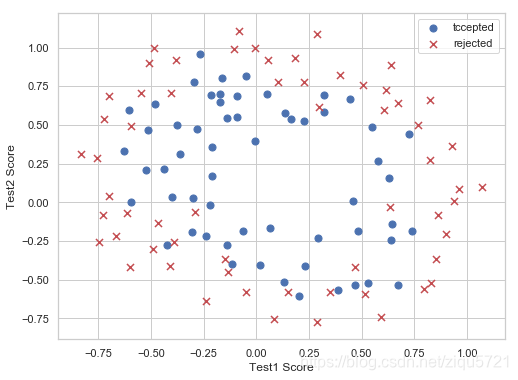
设想你是工厂的生产主管,你有一些芯片在两次测试中的测试结果。对于这两次测试,你想决定是否芯片要被接受或抛弃。为了帮助你做出艰难的决定,你拥有过去芯片的测试数据集,从其中你可以构建一个逻辑回归模型。
数据可视化
data2 = pd.read_csv('ex2data2.txt',header=None,names = ['test1','test2','accepted'])
data2.head()
| test1 | test2 | accepted | |
|---|---|---|---|
| 0 | 0.051267 | 0.69956 | 1 |
| 1 | -0.092742 | 0.68494 | 1 |
| 2 | -0.213710 | 0.69225 | 1 |
| 3 | -0.375000 | 0.50219 | 1 |
| 4 | -0.513250 | 0.46564 | 1 |
positive = data2[data2['accepted'].isin([1])]
negative = data2[data2['accepted'].isin([0])]

fig, ax = plt.subplots(figsize=(8,6))
ax.scatter(positive['test1'], positive['test2'], s=50, c='b', marker='o', label='tccepted')
ax.scatter(negative['test1'], negative['test2'], s=50, c='r', marker='x', label='rejected')
ax.legend()
ax.set_xlabel('Test1 Score')
ax.set_ylabel('Test2 Score')
Text(0, 0.5, 'Test2 Score')
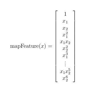
feature mapping(特征映射)
这个数据看起来可比前一次的复杂得多。特别地,你会注意到其中没有线性决策界限,来良好的分开两类数据。一个方法是用像逻辑回归这样的线性技术来构造从原始特征的多项式中得到的特征。
for i in 0..i
  for p in 0..i:
    output x^(i-p) * y^p
def feature_mapping(x, y, power, as_ndarray=False):

    data = {"f{}{}".format(i - p, p): np.power(x, i - p) * np.power(y, p)
                for i in np.arange(power + 1)
                for p in np.arange(i + 1)
            }

    if as_ndarray:
        return pd.DataFrame(data).as_matrix()
    else:
        return pd.DataFrame(data)
x1 = np.array(data2.test1)
x2 = np.array(data2.test2)
d = feature_mapping(x1, x2, power=6)
print(d.shape)
d.head()
(118, 28)
| f00 | f10 | f01 | f20 | f11 | f02 | f30 | f21 | f12 | f03 | ... | f23 | f14 | f05 | f60 | f51 | f42 | f33 | f24 | f15 | f06 | |
|---|---|---|---|---|---|---|---|---|---|---|---|---|---|---|---|---|---|---|---|---|---|
| 0 | 1.0 | 0.051267 | 0.69956 | 0.002628 | 0.035864 | 0.489384 | 0.000135 | 0.001839 | 0.025089 | 0.342354 | ... | 0.000900 | 0.012278 | 0.167542 | 1.815630e-08 | 2.477505e-07 | 0.000003 | 0.000046 | 0.000629 | 0.008589 | 0.117206 |
| 1 | 1.0 | -0.092742 | 0.68494 | 0.008601 | -0.063523 | 0.469143 | -0.000798 | 0.005891 | -0.043509 | 0.321335 | ... | 0.002764 | -0.020412 | 0.150752 | 6.362953e-07 | -4.699318e-06 | 0.000035 | -0.000256 | 0.001893 | -0.013981 | 0.103256 |
| 2 | 1.0 | -0.213710 | 0.69225 | 0.045672 | -0.147941 | 0.479210 | -0.009761 | 0.031616 | -0.102412 | 0.331733 | ... | 0.015151 | -0.049077 | 0.158970 | 9.526844e-05 | -3.085938e-04 | 0.001000 | -0.003238 | 0.010488 | -0.033973 | 0.110047 |
| 3 | 1.0 | -0.375000 | 0.50219 | 0.140625 | -0.188321 | 0.252195 | -0.052734 | 0.070620 | -0.094573 | 0.126650 | ... | 0.017810 | -0.023851 | 0.031940 | 2.780914e-03 | -3.724126e-03 | 0.004987 | -0.006679 | 0.008944 | -0.011978 | 0.016040 |
| 4 | 1.0 | -0.513250 | 0.46564 | 0.263426 | -0.238990 | 0.216821 | -0.135203 | 0.122661 | -0.111283 | 0.100960 | ... | 0.026596 | -0.024128 | 0.021890 | 1.827990e-02 | -1.658422e-02 | 0.015046 | -0.013650 | 0.012384 | -0.011235 | 0.010193 |
5 rows × 28 columns
# set X and y (remember from above that we moved the label to column 0)
cols = d.shape[1]
X2 = d.iloc[:,0:cols]
y2 = data2.iloc[:,-1]

# convert to numpy arrays and initalize the parameter array theta
X2 = np.array(X2.values)
y2 = np.array(y2.values)
theta2 = np.zeros(d.shape[1])
X2.shape
(118, 28)
regularized cost(正则化代价函数)
def regularized_cost(theta, X, y, l = 1):
#     '''you don't penalize theta_0'''
    theta_j1_to_n = theta[1:]
    regularized_term = (l / (2 * len(X))) * np.power(theta_j1_to_n, 2).sum()

    return cost(theta, X, y) + regularized_term
#正则化代价函数
regularized_cost(theta2, X2, y2)
81.79136730607354
注意等式中的"reg" 项。还注意到另外的一个“学习率”参数。这是一种超参数,用来控制正则化项。现在我们需要添加正则化梯度函数:
regularized gradient(正则化梯度)
def gradientReg(theta, X, y, l = 1):
    theta = np.matrix(theta)
    X = np.matrix(X)
    y = np.matrix(y)

    parameters = int(theta.ravel().shape[1])
    grad = np.zeros(parameters)

    error = sigmoid(X * theta.T) - y

    for i in range(parameters):
        term = np.multiply(error, X[:,i])

        if (i == 0):
            grad[i] = np.sum(term) / len(X)
        else:
            grad[i] = (np.sum(term) / len(X)) + ((l/ len(X)) * theta[:,i])

    return grad
gradientReg(theta2,X2,y2,l)
array([ 1.00000000e+00,  5.47789085e-02,  1.83101559e-01,  2.47575335e-01,
       -2.54718403e-02,  3.01369613e-01,  5.98333290e-02,  3.06815335e-02,
        1.54825117e-02,  1.42350013e-01,  1.22538429e-01, -5.25103811e-03,
        5.04328744e-02, -1.10481882e-02,  1.71098505e-01,  5.19650721e-02,
        1.18117999e-02,  9.43209446e-03,  1.82778085e-02,  4.08908411e-03,
        1.15709633e-01,  7.83711827e-02, -7.02782670e-04,  1.89334033e-02,
       -1.70495724e-03,  2.25916984e-02, -6.30180777e-03,  1.25725602e-01])
使用 scipy.optimize.minimize 去拟合参数
import scipy.optimize as opt
#print('init cost = {}'.format(regularized_cost(theta, X2, y2)))

res = opt.minimize(fun=regularized_cost, x0=theta2, args=(X2, y2), method='Newton-CG', jac=gradientReg)
res
     fun: 81.77441734193648
     jac: array([ 4.00721538e-05,  7.92107259e-06, -9.57130728e-06, -1.42508119e-05,
        4.85128609e-07,  1.45625425e-05,  3.29183446e-06, -8.83742842e-06,
       -1.54701906e-05,  6.29085218e-06,  3.15309983e-07, -1.77766493e-06,
       -1.69611923e-06,  4.61593901e-07,  2.27856315e-05,  9.39896102e-07,
       -6.13323667e-06, -5.07992963e-06,  4.76323762e-07, -1.47010548e-06,
        8.05396260e-06, -1.23147530e-06, -2.44197649e-06, -5.84739722e-07,
       -5.07920552e-07,  2.30737982e-07,  3.82757197e-06,  1.74447504e-05])
 message: "Warning: CG iterations didn't converge.  The Hessian is not positive definite."
    nfev: 7
    nhev: 0
     nit: 6
    njev: 1303
  status: 3
 success: False
       x: array([-3.39005803e-02,  1.10730363e-06,  9.39802365e-07, -6.09094336e-06,
        1.10972567e-06, -3.46309190e-06, -5.07574755e-06, -6.50187565e-06,
       -1.85556215e-06,  3.83480279e-06,  1.19556899e-05, -2.56049482e-06,
        1.03818042e-05,  7.10689627e-07, -1.07740558e-06,  6.38125479e-06,
        9.62469243e-06, -1.14576956e-06, -2.41930553e-06,  2.82923184e-06,
       -1.06295485e-05, -9.43499460e-06, -4.88500460e-07, -2.65549579e-06,
        4.89514367e-06, -5.46760048e-07, -4.56236184e-06,  9.44055863e-06])
final_theta =np.matrix(res.x)
predictions = predict(theta_min, X2)
correct = [1 if ((a == 1 and b == 1) or (a == 0 and b == 0)) else 0 for (a, b) in zip(predictions, y2)]
accuracy = (sum(map(int, correct)) % len(correct))
print ('accuracy = {0}%'.format(accuracy))
accuracy = 60%
使用不同的 (这个是常数)
画出决策边界
- 我们找到所有满足 的x
- instead of solving polynomial equation, just create a coridate x,y grid that is dense enough, and find all those that is close enough to 0, then plot them
def draw_boundary(power, l):
#     """
#     power: polynomial power for mapped feature
#     l: lambda constant
#     """
    density = 1000
    threshhold = 2 * 10**-3

    final_theta = feature_mapped_logistic_regression(power, l)
    x, y = find_decision_boundary(density, power, final_theta, threshhold)

    df = pd.read_csv('ex2data2.txt', names=['test1', 'test2', 'accepted'])
    sns.lmplot('test1', 'test2', hue='accepted', data=df, size=6, fit_reg=False, scatter_kws={"s": 100})

    plt.scatter(x, y, c='R', s=10)
    plt.title('Decision boundary')
def feature_mapped_logistic_regression(power, l):
#     """for drawing purpose only.. not a well generealize logistic regression
#     power: int
#         raise x1, x2 to polynomial power
#     l: int
#         lambda constant for regularization term
#     """
    df = pd.read_csv('ex2data2.txt', names=['test1', 'test2', 'accepted'])
    x1 = np.array(df.test1)
    x2 = np.array(df.test2)
    y =  df.iloc[:,-1]

    X = feature_mapping(x1, x2, power, as_ndarray=True)
    theta = np.zeros(X.shape[1])

    res = opt.minimize(fun=regularized_cost,
                       x0=theta,
                       args=(X, y, l),
                       method='TNC',
                       jac=gradientReg)
    final_theta = res.x

    return final_theta
def find_decision_boundary(density, power, theta, threshhold):
    t1 = np.linspace(-1, 1.5, density)
    t2 = np.linspace(-1, 1.5, density)

    cordinates = [(x, y) for x in t1 for y in t2]
    x_cord, y_cord = zip(*cordinates)
    mapped_cord = feature_mapping(x_cord, y_cord, power)  # this is a dataframe

    inner_product = mapped_cord.as_matrix() @ theta

    decision = mapped_cord[np.abs(inner_product) < threshhold]

    return decision.f10, decision.f01
#寻找决策边界函数
draw_boundary(power=6, l=0)#lambda=1

draw_boundary(power=6, l=0) # no regularization, over fitting,#lambda=0,没有正则化,过拟合了

draw_boundary(power=6, l=100) # underfitting,#lambda=100,欠拟合

调用sklearn的线性回归包
from sklearn import linear_model
model = linear_model.LogisticRegression(penalty='l2', C=1.0)
model.fit(X2, y2.ravel())
LogisticRegression(C=1.0, class_weight=None, dual=False, fit_intercept=True,
          intercept_scaling=1, max_iter=100, multi_class='warn',
          n_jobs=None, penalty='l2', random_state=None, solver='warn',
          tol=0.0001, verbose=0, warm_start=False)
model.score(X2, y2)
0.8305084745762712