04-autograd与逻辑回归

一、自动求导（autograd）

1.1 torch.autograd.backward

torch.autograd.backward(tensors, grad_tensors=None, retain_graph=None,create_graph=False)

功能：自动求取梯度

• tensors: 用于求导的张量,如loss
• retain_graph : 保存计算图
• create-graph: 创建导数计算图,用于高阶求导
• grad_tensors: 多梯度权重的设置,用于多维loss

# -*- coding:utf-8 -*-
import torch

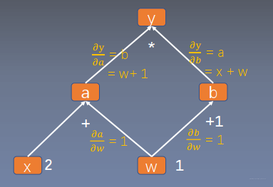
w = torch.tensor([1.], requires_grad=True)
x = torch.tensor([2.], requires_grad=True)

a = torch.add(w, x)
b = torch.add(w, 1)
y = torch.mul(a, b)

# 通过设置retain_graph=True，来再次使用计算图
y.backward(retain_graph=True) 
print(w.grad)
y.backward()

注意： 计算图在第一次使用过后，会被系统释放掉，如果还想再次使用，则需要设置retain_graph=True

# -*- coding:utf-8 -*-
import torch

w = torch.tensor([1.], requires_grad=True)
x = torch.tensor([2.], requires_grad=True)

a = torch.add(w, x)  # retain_grad()
b = torch.add(w, 1)

y0 = torch.mul(a, b)  # y0 = (x+w) * (w+1)
y1 = torch.add(a, b)  # y1 = (x+w) + (w+1)    dy1/dw = 2

loss = torch.cat([y0, y1], dim=0)  # [y0, y1]
grad_tensors = torch.tensor([1., 2.])

loss.backward(gradient=grad_tensors)  # gradient 传入 torch.autograd.backward()中的grad_tensors

print(w.grad)

说明： 当损失函数维为多维时，可以通过设置 grad_tensors来设置每一维的权重，最终的损失维每一维的加权和

1.2 torch.autograd.grad

torch.autograd.grad(outputs,inputs,grad_outputs=None,retain graph=None,create_graph=False)

功能：求取梯度

• outputs: 用于求导的张量,如loss
• inputs: 需要梯度的张量
• create_graph: 创建导数计算图,用于高阶求导
• retain_graph: 保存计算图
• grad_outputs: 多梯度权重

x = torch.tensor([3.], requires_grad=True)
y = torch.pow(x, 2)  # y = x**2

grad_1 = torch.autograd.grad(y, x, create_graph=True)  # grad_1 = dy/dx = 2x = 2 * 3 = 6
print(grad_1)

grad_2 = torch.autograd.grad(grad_1[0], x)  # grad_2 = d(dy/dx)/dx = d(2x)/dx = 2
print(grad_2)

注意：

1. 梯度不自动清零
2. 依赖于叶子结点的结点, requires-grad默认为True
3. 叶子结点不可执行in-place操作

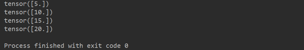
# 梯度不自动清零
w = torch.tensor([1.], requires_grad=True)
x = torch.tensor([2.], requires_grad=True)

for i in range(4):
    a = torch.add(w, x)
    b = torch.add(w, 1)
    y = torch.mul(a, b)

    y.backward()
    print(w.grad)

    # w.grad.zero_() # 手动设置对梯度清理

# 依赖于叶子结点的结点, requires-grad默认为True
w = torch.tensor([1.], requires_grad=True)
x = torch.tensor([2.], requires_grad=True)

a = torch.add(w, x)
b = torch.add(w, 1)
y = torch.mul(a, b)

print(a.requires_grad, b.requires_grad, y.requires_grad)

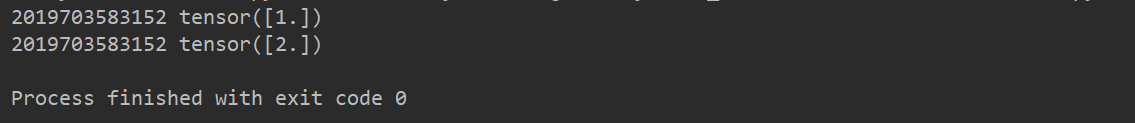
# in-place操作
a = torch.ones((1,))
print(id(a), a)

# a = a + torch.ones((1, ))
# print(id(a), a)

a += torch.ones((1,))  # in-place操作，处理的是同一块内存地址
print(id(a), a)

叶子结点不可执行in-place操作的原因：

反向传播计算叶子结点w的梯度时，需要计算 $\frac{\partial y}{\partial a}$，而 $\frac{\partial y}{\partial a}=w+1$，需要用到叶子结点w，在前向转播过程记录了w的地址，然后根据该地址，才能在反向传播过程中找到w的数据，所以如果在反向传播之前改变了该地址当中的数据，则反向传播计算梯度则会出错

二、逻辑回归

逻辑回归是线性的二分类模型，是分析自变量x与**因变量y(概率)**之间关系的方法

模型表达式： $y=f(wx+b)$
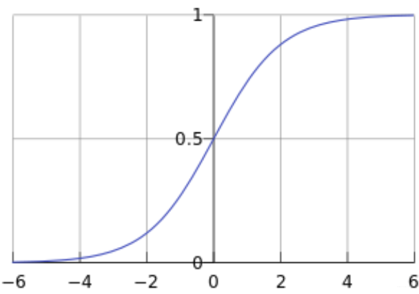
其中， $f(x)=\frac{1}{1+e^{-x}}$， $f(x)$称为Sigmoid函数，也称为Logistic函数

机器学习模型训练步骤

1. 数据
2. 模型
3. 损失函数
4. 优化器
5. 迭代训练

# ============================ step 1/5 生成数据 ============================
sample_nums = 100
mean_value = 1.7
bias = 1
n_data = torch.ones(sample_nums, 2)
x0 = torch.normal(mean_value * n_data, 1) + bias      # 类别0 数据 shape=(100, 2)
y0 = torch.zeros(sample_nums)                         # 类别0 标签 shape=(100, 1)
x1 = torch.normal(-mean_value * n_data, 1) + bias     # 类别1 数据 shape=(100, 2)
y1 = torch.ones(sample_nums)                          # 类别1 标签 shape=(100, 1)
train_x = torch.cat((x0, x1), 0)
train_y = torch.cat((y0, y1), 0)


# ============================ step 2/5 选择模型 ============================
class LR(nn.Module):
    def __init__(self):
        super(LR, self).__init__()
        self.features = nn.Linear(2, 1)
        self.sigmoid = nn.Sigmoid()

    def forward(self, x):
        x = self.features(x)
        x = self.sigmoid(x)
        return x


lr_net = LR()   # 实例化逻辑回归模型


# ============================ step 3/5 选择损失函数 ============================
loss_fn = nn.BCELoss()

# ============================ step 4/5 选择优化器   ============================
lr = 0.01  # 学习率
optimizer = torch.optim.SGD(lr_net.parameters(), lr=lr, momentum=0.9)

# ============================ step 5/5 模型训练 ============================
for iteration in range(1000):

    # 前向传播
    y_pred = lr_net(train_x)

    # 计算 loss
    loss = loss_fn(y_pred.squeeze(), train_y)

    # 反向传播
    loss.backward()

    # 更新参数
    optimizer.step()

    # 清空梯度
    optimizer.zero_grad()

    # 绘图
    if iteration % 20 == 0:

        mask = y_pred.ge(0.5).float().squeeze()  # 以0.5为阈值进行分类
        correct = (mask == train_y).sum()  # 计算正确预测的样本个数
        acc = correct.item() / train_y.size(0)  # 计算分类准确率

        plt.scatter(x0.data.numpy()[:, 0], x0.data.numpy()[:, 1], c='r', label='class 0')
        plt.scatter(x1.data.numpy()[:, 0], x1.data.numpy()[:, 1], c='b', label='class 1')

        w0, w1 = lr_net.features.weight[0]
        w0, w1 = float(w0.item()), float(w1.item())
        plot_b = float(lr_net.features.bias[0].item())
        plot_x = np.arange(-6, 6, 0.1)
        plot_y = (-w0 * plot_x - plot_b) / w1

        plt.xlim(-5, 7)
        plt.ylim(-7, 7)
        plt.plot(plot_x, plot_y)

        plt.text(-5, 5, 'Loss=%.4f' % loss.data.numpy(), fontdict={'size': 20, 'color': 'red'})
        plt.title("Iteration: {}\nw0:{:.2f} w1:{:.2f} b: {:.2f} accuracy:{:.2%}".format(iteration, w0, w1, plot_b, acc))
        plt.legend()

        plt.show()
        plt.pause(0.5)

        if acc > 0.99:
            break