pytorch学习--autograd与逻辑回归

自动求导autograd与逻辑回归

torch.autograd

torch.autograd.backward(tensors,gradient=None,retain_graph=None,create_graph=False
tensors:用于求导的张量，如loss
retain_graph:用于保存计算图
create_graph:用于创建导数计算图，用于高阶求导
gradient:多梯度权重

y=(x+w)*(w+1)
a=x+w b=w+1
y=ab

y对w求导:
∂y/∂w=（∂y/∂a）*（∂a/∂w）+(∂y/∂b)*(∂b\∂w)
=b*1+a*1
=b+a
=(w+1)+(x+w)
=2*w+x+1

w初值为1 x为2 梯度为5

import torch

w=torch.tensor([1.],requires_grad=True)  #求梯度的 必须是浮点数类型
x=torch.tensor([2.],requires_grad=True)

a=torch.add(x,w)
b=torch.add(w,1)
y=torch.mul(a,b)
#反向传播
y.backward()  #实际上调用的就是autograd.backward()
#调用一次backward之后 会将计算图清空   所以当再调用一次backward() 会出错 所以
#y.backward(retain_graph=True)
print(w.grad)  #5

多梯度权重的设置

import torch

w=torch.tensor([1.],requires_grad=True)
x=torch.tensor([2.],requires_grad=True)

a=torch.add(x,w)
b=torch.add(w,1)

y0=torch.mul(a,b)
y1=torch.add(a,b)
loss=torch.cat([y0,y1],dim=0)
#设置多个权重值  y0的权重为1  y1的权重为2
grad_tensors=torch.tensor([1.,2.])
loss.backward(gradient=grad_tensors)
print(w.grad)

torch.autograd.grad(outputs,inputs,grad_outputs=None,retain_graph=None,create_graph=False)
outputs:用于求导的张量，如loss
inputs :需要梯度的张量
create_graph:创建导数计算图，用于高阶求导
retain_graph:保存计算图

autograd小贴士

1梯度不自动清零

必须要进行手动清零 如果不清零的话会一直累加
清零操作:w.grad.zero_()

2.依赖于叶子结点的结点，requires_grad默认为True
3.叶子节点不可以执行in-place

逻辑回归

逻辑回归是线性的二分类模型
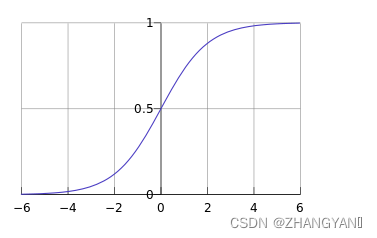
y=f(w*x+b)
f(x)=1/(1+e^-x)
f(x)是Sigmoid函数 ，也称为logistic函数

训练的五个步骤：数据、模型、损失函数、优化器、迭代训练。

# ============================ step 1/5 生成数据 ============================
sample_nums = 100
mean_value = 1.7
bias = 1
n_data = torch.ones(sample_nums, 2)
x0 = torch.normal(mean_value * n_data, 1) + bias  # 正态分布  类别0 数据 shape=(100, 2)
y0 = torch.zeros(sample_nums)  # 类别0 标签 shape=(100, 1)
x1 = torch.normal(-mean_value * n_data, 1) + bias  # 类别1 数据 shape=(100, 2)
y1 = torch.ones(sample_nums)  # 类别1 标签 shape=(100, 1)
train_x = torch.cat((x0, x1), 0)
train_y = torch.cat((y0, y1), 0)
print(x0)
# ============================ step 2/5 选择模型 ============================
class LR(nn.Module):
    def __init__(self):
        super(LR, self).__init__()
        self.features = nn.Linear(2, 1)
        self.sigmoid = nn.Sigmoid()
    #前向传播
    def forward(self, x):
        x = self.features(x)
        x = self.sigmoid(x)
        return x
lr_net = LR()  # 实例化逻辑回归模型

# ============================ step 3/5 选择损失函数 ============================
loss_fn = nn.BCELoss()  # 二分类常使用的交叉商函数

# ============================ step 4/5 选择优化器   ============================
lr = 0.01  # 学习率
optimizer = torch.optim.SGD(lr_net.parameters(), lr=lr, momentum=0.9)

# ============================ step 5/5 模型训练 ============================
for iteration in range(1000):

    # 前向传播
    y_pred = lr_net(train_x)

    # 计算 loss
    loss = loss_fn(y_pred.squeeze(), train_y)

    # 反向传播
    loss.backward()

    # 更新参数
    optimizer.step()

    # 清空梯度
    optimizer.zero_grad()

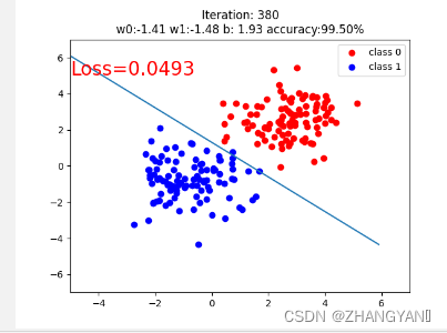
    # 绘图
    if iteration % 20 == 0:

        mask = y_pred.ge(0.5).float().squeeze() # 以0.5为阈值进行分类
        # print(mask)
        correct = (mask == train_y).sum()  # 计算正确预测的样本个数
        acc = correct.item() / train_y.size(0)  # 计算分类准确率

        plt.scatter(x0.data.numpy()[:, 0], x0.data.numpy()[:, 1], c='r', label='class 0')
        plt.scatter(x1.data.numpy()[:, 0], x1.data.numpy()[:, 1], c='b', label='class 1')
        
        w0, w1 = lr_net.features.weight[0]

        w0, w1 = float(w0.item()), float(w1.item())
        plot_b = float(lr_net.features.bias[0].item())
        plot_x = np.arange(-6, 6, 0.1)
        plot_y = (-w0 * plot_x - plot_b) / w1

        plt.xlim(-5, 7)
        plt.ylim(-7, 7)
        plt.plot(plot_x, plot_y)

        plt.text(-5, 5, 'Loss=%.4f' % loss.data.numpy(), fontdict={'size': 20, 'color': 'red'})
        plt.title("Iteration: {}\nw0:{:.2f} w1:{:.2f} b: {:.2f} accuracy:{:.2%}".format(iteration, w0, w1, plot_b, acc))
        plt.legend()

        plt.show()
        plt.pause(0.5)

        if acc > 0.99:
            break