深度学习 -- pytorch 计算图与动态图机制 autograd与逻辑回归模型

前言

pytorch中的动态图机制是pytorch这门框架的优势所在，阅读本篇博客可以使我们对动态图机制以及静态图机制有更直观的理解，同时在博客的后半部分有关于逻辑回归的知识点，并且使用pytorch中张量以及张量的自动求导进行构建逻辑回归模型。

计算图

计算图是用来描述运算的有向无环图

计算图有两个主要元素:节点（Node）和边（Edge）

节点表示数据，如向量，矩阵，张量，边表示运算，如加减乘除卷积等。

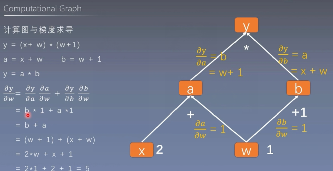
用计算图表示：y = (x+w)*(w+1)

• a = x + w
• b = w + 1
• y = a * b

采用计算图进行计算的好处

它不仅仅能够让我们的运算更加简洁，更重要的作用是使得梯度求导更方便

我们可以用pytorch模拟这个过程

import torch

# 创建w和x两个节点
w = torch.tensor([1.],requires_grad=True)
x = torch.tensor([2.],requires_grad=True)

a = torch.add(w,x)
b = torch.add(w,1)
y = torch.mul(a,b)

y.backward()  # 调用反向传播 梯度求导
print(w.grad)  # tensor([5.])

叶子节点

用户创建的节点称为叶子节点
上述代码创建的w和x 就是叶子节点
is_leaf:知识张量是否为叶子结点

• 只有叶子节点能输出梯度 因为非叶子节点在计算之后的梯度会自动回收

import torch

# 创建w和x两个节点
w = torch.tensor([1.],requires_grad=True)
x = torch.tensor([2.],requires_grad=True)

a = torch.add(w,x)
b = torch.add(w,1)
y = torch.mul(a,b)

# y.backward()  # 调用反向传播 梯度求导
# print(w.grad)
print(w.is_leaf,x.is_leaf,a.is_leaf,b.is_leaf,y.is_leaf)

输出：

True True False False False

输出非叶子节点的梯度的方法

在非叶子节点创建之后执行.retain_grad()命令

import torch

# 创建w和x两个节点
w = torch.tensor([1.],requires_grad=True)
x = torch.tensor([2.],requires_grad=True)

a = torch.add(w,x)
a.retain_grad()
b = torch.add(w,1)
y = torch.mul(a,b)

y.backward()  # 调用反向传播 梯度求导
# print(w.grad)
# print(w.is_leaf,x.is_leaf,a.is_leaf,b.is_leaf,y.is_leaf)
print(w.grad,a.grad)  # tensor([5.]) tensor([2.])

• grad_fn:记录创建该张量时所用的方法

print(y.grad_fn,a.grad_fn,b.grad_fn)
# 输出：
# <MulBackward0 object at 0x0000026458E32CA0>
# <AddBackward0 object at 0x0000026458DA2670> 
# <AddBackward0 object at 0x0000026458DA20D0>

动态图与静态图

在计算图中，根据搭建方式的不同，可以将计算图分为动态图和静态图。

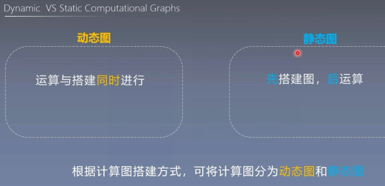
动态图的优点：灵活、易调节
静态图的优点：高效
静态图的缺点：不灵活

pytorch中的自动求导系统autograd

torch.autograd

梯度的计算在模型训练中是十分重要的，然而梯度的计算十分的繁琐，所以pytorch提供了一套自动求导的系统，我们只需要手动搭建计算图，pytorch就能帮我们自动求导。

• torch.autograd.backward

功能：自动求取梯度

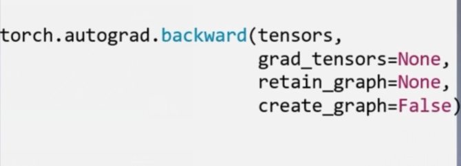
tensors:用于求导的张量，如loss
retain_graph:保存计算图
create_graph:创建导数计算图，用于高阶求导
grad_tensors：多梯度权重

张量中的backward()方法实际就是调用了atuograd.backward()方法

y.backward(retain_graph=True)

backward方法中的参数retain_graph，是保存计算图的意思，如果想要连续进行两次反向传播，这个参数必须设置为True，因为如果用默认的false，执行完第一次之后pytorch会把计算图自动释放掉。

grad_tensors的使用

import torch

# 创建w和x两个节点
w = torch.tensor([1.],requires_grad=True)
x = torch.tensor([2.],requires_grad=True)

a = torch.add(w,x)
a.retain_grad()
b = torch.add(w,1)
y0 = torch.mul(a,b)
y1 = torch.add(a,b)
loss = torch.cat([y0,y1],dim=0)
grad_tensors = torch.tensor([1.,1.])
loss.backward(gradient=grad_tensors)
print(w.grad)  # tensor([7.])

• torch.atuograd.grad

功能：求取梯度

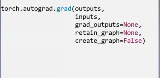
outputs:用于求导的张量，如loss
inputs:需要梯度的张量
create_graph：创建导数计算图，用于高阶求导
retain_graph:保存计算图
grad_outputs:多梯度权重

高阶导数

import torch
x = torch.tensor([3.],requires_grad=True)
y = torch.pow(x,2) # y = x**2

# 1阶求导 对y进行求导
grad_1 = torch.autograd.grad(y,x,create_graph=True) # create_graph：创建导数计算图，用于高阶求导
print(grad_1)  # (tensor([6.], grad_fn=<MulBackward0>),)


# 2阶求导
grad_2 = torch.autograd.grad(grad_1[0],x)
print(grad_2) # (tensor([2.]),)

注意：
1、梯度不自动清零

import torch
w = torch.tensor([1.],requires_grad=True)
x = torch.tensor([2.],requires_grad=True)

for i in range(4):
    a = torch.add(w,x)
    b = torch.add(w,1)
    y = torch.mul(a,b)

    y.backward()
    print(w.grad)
    

输出：

tensor([5.])
tensor([10.])
tensor([15.])
tensor([20.])

说明梯度是不断累加的，原位操作 .grad.zero_() 就能解决这个问题

2、依赖于叶子结点的结点的require_grad都是True

import torch

# 创建w和x两个节点
w = torch.tensor([1.],requires_grad=True)
x = torch.tensor([2.],requires_grad=True)

a = torch.add(w,x)
a.retain_grad()
b = torch.add(w,1)
y0 = torch.mul(a,b)
y1 = torch.add(a,b)
loss = torch.cat([y0,y1],dim=0)
grad_tensors = torch.tensor([1.,1.])
loss.backward(gradient=grad_tensors)
print(a.requires_grad,b.requires_grad,y0.requires_grad,y1.requires_grad)
# True True True True

3、叶子结点不可执行in-place操作（原位操作）

import torch

# 创建w和x两个节点
w = torch.tensor([1.],requires_grad=True)
x = torch.tensor([2.],requires_grad=True)

a = torch.add(w,x)
a.retain_grad()
b = torch.add(w,1)
y0 = torch.mul(a,b)
y1 = torch.add(a,b)
w.add_(1)

报错信息：

    w.add_(1)
RuntimeError: a leaf Variable that requires grad is being used in an in-place operation.

原位操作：在原始地址上直接进行改变

逻辑回归

逻辑回归模型是线性的二分类模型
模型表达式：
y = f(WX + b)
f(x) = 1/(1+e**-x)

f(x) 称为Sigmoid函数，也称为logistic函数

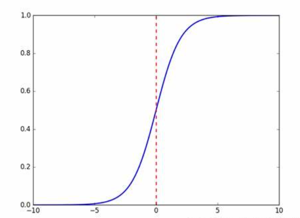
这样的函数我们通过设定一个阈值来进行二分类的工作

比如：当y的值小于等于0>=0.5 则最终输出1，反之则输出0。

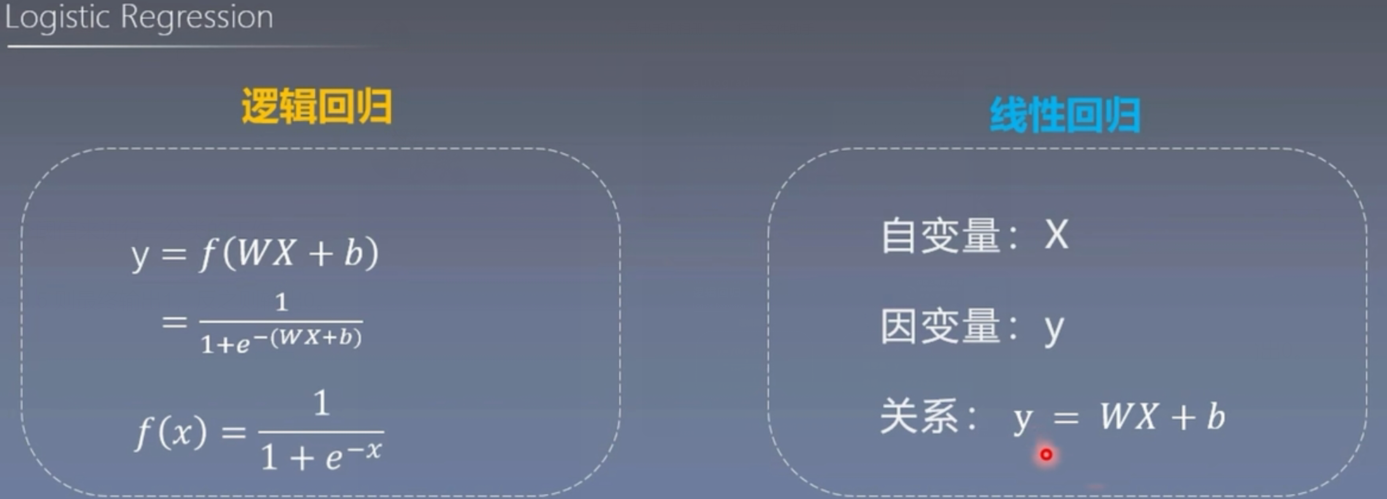
线性回归是分析自变量x与因变量y(标量)之间的关系的方法
逻辑回归是分析自变量x与因变量y(概率)之间的关系的方法

pytorch中构建逻辑回归模型

import torch
import torch.nn as nn
import matplotlib.pyplot as plt
import numpy as np


# 步骤1 生成数据
sample_nums = 100
mean_value = 1.7
bias = 1
n_data = torch.ones(sample_nums,2)
x0 = torch.normal(mean_value*n_data,1)+bias     # 类别0的数据 shape=(100,2)
y0 = torch.zeros(sample_nums)           # 类别0的数据 shape=(100，1)
x1 = torch.normal(-mean_value*n_data,1)+bias # 类别1的数据 shape(100,2)
y1 = torch.ones(sample_nums)            # 类别为1 标签 shape(100,1)
train_x = torch.cat((x0,x1),0)
train_y = torch.cat((y0,y1),0)

# 步骤2 选择模型
class LR(nn.Module):
    def __init__(self):
        super(LR,self).__init__()
        self.features = nn.Linear(2,1)
        self.sigmoid = nn.Sigmoid()

    def forward(self,x):
        x = self.features(x)
        x = self.sigmoid(x)
        return x

lr_net = LR() # 实例化逻辑回归模型

# 步骤3 选择损失函数
loss_fn = nn.BCELoss() # 交叉熵

# 步骤4 选择损失函数
lr = 0.01  # 学习率
optimizer = torch.optim.SGD(lr_net.parameters(),lr=lr,momentum=0.9)

# 步骤5 模型训练
for interation in range(1000):
    # 前向传播
    y_pred = lr_net(train_x)

    # 计算损失
    loss = loss_fn(y_pred.squeeze(),train_y)

    # 反向传播
    loss.backward()

    # 更新参数
    optimizer.step()

    # 绘图
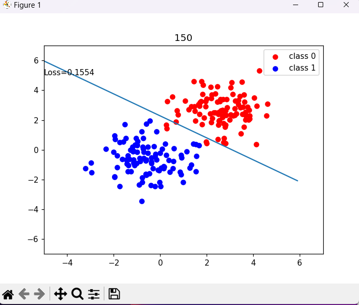
    if interation % 50==0:

        mask = y_pred.ge(0.5).float().squeeze() # 以0.5为阈值进行分类
        correct = (mask == train_y).sum()
        acc = correct.item()/train_y.size(0)

        plt.scatter(x0.data.numpy()[:,0],x0.data.numpy()[:,1],c="r",label="class 0")
        plt.scatter(x1.data.numpy()[:,0],x1.data.numpy()[:,1],c="b",label="class 1")

        w0,w1 = lr_net.features.weight[0]
        w0,w1 = float(w0.item()),float(w1.item())
        plot_b = float(lr_net.features.bias[0].item())
        plot_x = np.arange(-6,6,0.1)
        plot_y = (-w0*plot_x - plot_b)/w1

        plt.xlim(-5,7)
        plt.ylim(-7,7)
        plt.plot(plot_x,plot_y)

        plt.text(-5,5,'Loss=%.4f'%loss.data.numpy())
        plt.title(interation)

        plt.legend()

        plt.show()

        if acc > 0.99:
            break