机器学习基石笔记（四）：学习的可行性

Lecture 4: Feasibility of Learning

Learning is Impossible?

  absolutely no free lunch outside $D​$

No Free Lunch

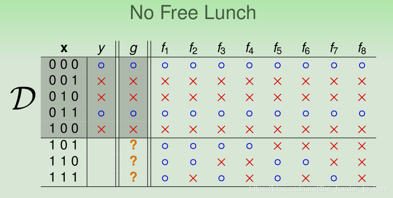
在已知的样本( $D_x$)中， $f_1 \sim f_8$都符合( $y_x=g_x$)，但不同的f所预测的y完全不同。

你不能说这八个模型中谁比谁好，也就是说这八个模型预测都是对的，

Fun Time

This is a popular ‘brain-storming’ problem, with a claim that 2% of the world’s cleverest population can crack its ‘hidden pattern’.
$(5,3,2) → 151022, (7,2,5) → ?$
It is like a ‘learning problem’ with $N = 1, x_1 = (5,3,2), y_1 = 151022$.
Learn a hypothesis from the one example to predict on x = (7,2,5).
What is your answer?
1 151026
2 143547
3 I need more examples to get the correct answer
4 there is no ‘correct’ answer   $\checkmark$


Explanation
根据“没有免费的午餐”，我们根据有限的输入，理论上在输入外可以得到一定数量的等价模型。
所以输入越多，归纳得到的规律 $f$就越靠近 $g$。
但是实际上我们永远得不到g，除非你拥有所有的样本（但如果你拥有所有的样本，直接对比查询即可，用不着用模型模拟了）或者加上其他的条件/倾向。


? 所以说数列要写通项公式才规范，小时候写的数学规律题目其实都不严谨，因为我发现一道填空题可能有多个答案，而标准答案往往只给一个。

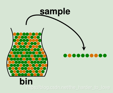
Probability to the Rescue

我们使用统计学与概率论工具，用已知样本的分布预估未知样本的分布。简单来说类似于抽样检测（实际上我们所做的相反：用样本估计整体），如下图所示。

Hoeffding’s Inequality

   In big sample ( $N$ large), $ν$ is probably close to $µ$ (within $\epsilon$)
$\mathbb{P}[|\nu-\mu|>\epsilon] \leq 2 \exp \left(-2 \epsilon^{2} N\right)$
   for marbles, coin, polling, …
   概率上界的大小取决于宽松间隙( $\epsilon$)和样本数量( $N$)，两者越大，概率上界就越小。
   $\nu \approx \mu$，概率最大，接近1.
   $N$越大，越有可能用 $\nu$推测 $\mu​$

Fun Time

Let $\mu$ = 0.4. Use Hoeffding’s Inequality
$\mathbb{P}[|\nu-\mu|>\epsilon] \leq 2 \exp \left(-2 \epsilon^{2} N\right)$
to bound the probability that a sample of 10 marbles will have $\nu ≤ 0.1$. What bound do you get?
1 0.67
2 0.40
3 0.33   $\checkmark​$
4 0.05


Explanation
$|\nu-\mu| \ge 0.3 \\ \therefore \epsilon=0.3 \\ 又 \, N=10 \\ bound = 0.3305977764431732$

? 霍夫丁不等式告诉了数据之间差距的概率上界，若知道数据的概率分布(概率密度函数|分布列)，可积分直接求出概率。
霍夫丁不等式是统计学和概率论中最重要的几个定理之一。

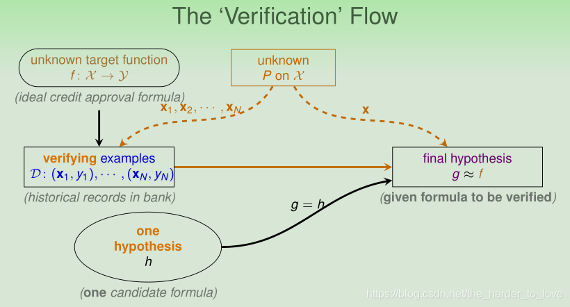
Connection to Learning

${E_{\text { in }}(\mathrm{h})=\frac{1}{N} \sum_{n=1}^{N}\left[h\left(\mathbf{x}_{n}\right) \neq y_{n}\right]} \Rightarrow {E_{\text { out }}(\mathrm{h})=\underset{\mathbf{x} \sim P}{\mathcal{E}}[h(\mathbf{x}) \neq f(\mathbf{x})]}$

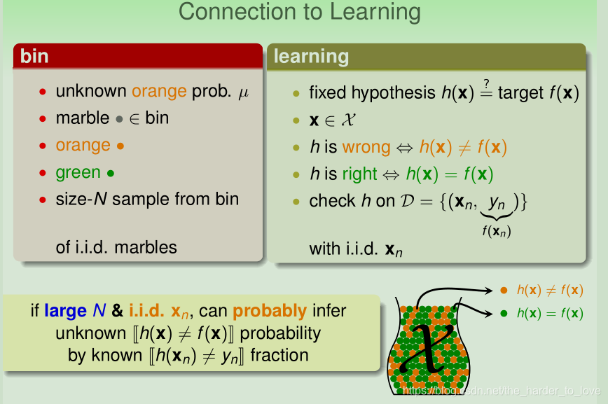
如果 $N$足够大，我们可以用 $E_{in}(h)$(in-sample error)来估计 $E_{out}(h)​$(out-sample error)。

$\mathbb{P}\left[ | E_{\text { in }}(h)-E_{\text { out }}(h) |>\epsilon\right] \leq 2 \exp \left(-2 \epsilon^{2} N\right)$

$\forall \ big \ N, \ small \ \mathcal{E} \\ E_{\mathrm{in}}(h) \approx E_{\mathrm{out}}(h) \\ E_{\mathrm{in}}(h) \ small \Rightarrow g \approx f \\ E_{\mathrm{in}}(h) \ not \ small \Rightarrow g \neq f$

Fun Time

Your friend tells you her secret rule in investing in a particular stock: ‘Whenever the stock goes down in the morning, it will go up in the afternoon;vice versa.’
To verify the rule, you chose 100 days uniformly at random from the past 10 years of stock data, and found that 80 of them satisfy the rule.
What is the best guarantee that you can get from the verification?
1 You’ll definitely be rich by exploiting the rule in the next 100 days.
2 You’ll likely be rich by exploiting the rule in the next 100 days, if the market behaves similarly to the last 10 years.   $\checkmark​$
3 You’ll likely be rich by exploiting the ‘best rule’ from 20 more friends in the next 100 days.
4 You’d definitely have been rich if you had exploited the rule in the past 10 years.


Explanation
股票市场风云变幻，你用历史数据搭建了一个优秀的模型当且仅当未来的趋势跟历史发展一致时，你才能利用这个模型获益。
从霍夫丁不等式的角度来看：历史数据搭建了一个优秀的模型( $E_{\mathrm{in}}(h) \ small​$), 且未来的趋势跟历史发展一致时 $E_{\mathrm{in}}(h) \approx E_{\mathrm{out}}(h)​$，那么模型对于未来趋势预测的效果优秀( $E_{\mathrm{out}}(h) \ small​$)，你最终就能获益。

Connection to Real Learning

之前是验证1个假设，别忘了，我们的假设集有多个假设，来看看真实的学习环境下，霍夫丁不等式应用的改变。

Multiple h

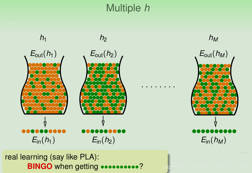
假设现在有150名同学，每人抛五次硬币，问出现连续朝上五枚硬币的概率是多少？
$1-\left(\frac{31}{32}\right)^{150} = 99.145 \%$
由于同学数量高达150名，出现连续朝上五枚硬币的概率达到 $99$，倘若我们用硬币全部朝上的数据而选择一直猜硬币朝上， $E_in = 0$ and $E_out = \frac{1}{2}$

BAD Sample and BAD Data

由于假设集增多，极端数据出现的可能性增大，由于我们的选择，导致 $E_{in}$ and $E_{out}$差别过大，我们将这样的选择称为 $Bad \ Sample$.

$E_{out}$ big (far from $f$), but $E_{in}​$ small (correct on most examples) called BAD Data.

$\mathbb{P}_{\mathcal{D}}[\mathrm{BAD} \ \mathcal{D}]=\sum_{\text { all possible } \mathcal{D}} \mathbb{P}(\mathcal{D}) \cdot[\mathrm{BAD} \ \mathcal{D}]$

$$ \begin{aligned} \ \mathbb{P}_{\mathcal{D}}[\mathrm{BAD} \ \mathcal{D}] & = \mathbb{P}_{\mathcal{D}}[\mathrm{BAD} \ \mathcal{D} \ for \ h_1 \ or \ \mathrm{BAD} \ \mathcal{D} \ for \ h_2 \ or \ ... \ or \ \mathrm{BAD} \ \mathcal{D} \ for \ h_M] \\ \ & \le \mathbb{P}_{\mathcal{D}}[\mathrm{BAD} \ \mathcal{D} \ for \ h_1]+\mathbb{P}_{\mathcal{D}}[\mathrm{BAD} \ \mathcal{D} \ for \ h_2]+...+\mathbb{P}_{\mathcal{D}}[\mathrm{BAD} \ \mathcal{D} \ for \ h_M](union \ bound) \\ \ & \leq 2 \exp \left(-2 \epsilon^{2} N\right)+2 \exp \left(-2 \epsilon^{2} N\right)+\ldots+2 \exp \left(-2 \epsilon^{2} N\right) \\ \ & {=2 M \exp \left(-2 \epsilon^{2} N\right)} \end{aligned} $$

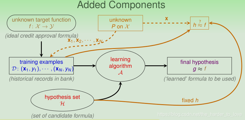
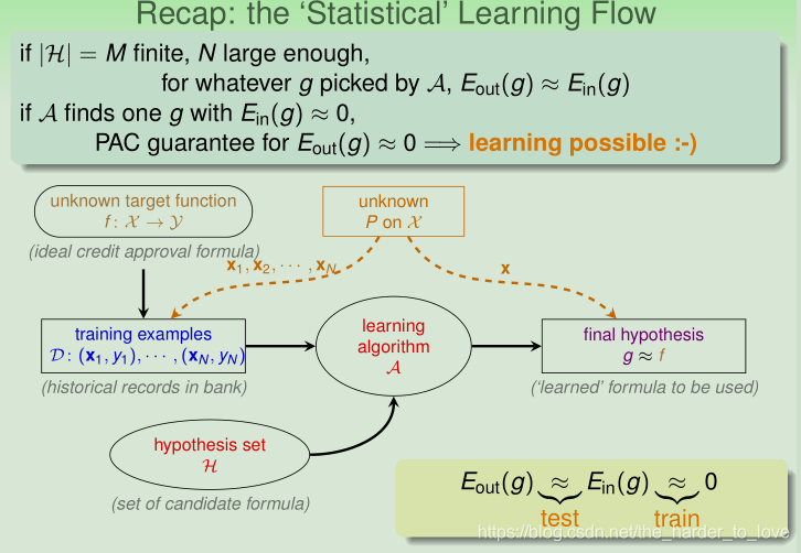
The ‘Statistical’ Learning Flow

若假设集( $|H|$)大小为有限的 $M$， $N$足够大，通过机器学习演算法( $A$)学习到的对于任意一个 $g$，都有 $E_{\mathrm{in}}(g) \approx E_{\mathrm{out}}(g)$.
若此时 $A$学到一个 $E_{\mathrm{in}}(g) \approx 0$，就能保证 $E_{\mathrm{out}}(g) \approx 0​$ => learning impossible 真正学到了知识:-).

Fun Time

Consider 4 hypotheses.
$\begin {array}{c}{h_{1}(\mathbf{x})=\operatorname{sign}\left(x_{1}\right), \quad h_{2}(\mathbf{x})=\operatorname{sign}\left(x_{2}\right)} \\ {h_{3}(\mathbf{x})=\operatorname{sign}\left(-x_{1}\right), \quad h_{4}(\mathbf{x})=\operatorname{sign}\left(-x_{2}\right)}\end{array}$
For any $N$ and $\epsilon$, which of the following statement is not true?
1 the BAD data of $h_1$ and the BAD data of $h_2$ are exactly the same.   $\checkmark$
2 the BAD data of $h_1$ and the BAD data of $h_3$ are exactly the same.
3 $\mathbb{P_D}[\mathrm{BAD} \ for \ some \ h_k] \leq 8 \exp \left(-2 \epsilon^{2} N\right)$
4 $\mathbb{P_D}[\mathrm{BAD} \ for \ some \ h_k] \leq 4 \exp \left(-2 \epsilon^{2} N\right)$


Explanation
参考多个 $g$中，霍夫丁不等式的上界推导公式。
对于BAD data $x$， $E_{in}$和 $E_{out}$相差大，那么假设h对于 $-x$，所得到 $-E_{in}$和 $-E_{out}$相差也会大，所以 $x$和 $-x$都是BAD data.
所以 $\operatorname{sign}\left(x_{}\right)$和 $\operatorname{sign}\left(-x_{}\right)$有相同的BAD data.

Summary

讲义总结

假设集( $|H|$)大小为有限的 $M$， $N$足够大，通过机器学习演算法( $A$)学习到的对于任意一个 $g$，都有 $E_{\mathrm{in}}(g) \approx E_{\mathrm{out}}(g)$.
若此时 $A$学到一个 $E_{\mathrm{in}}(g) \approx 0$，就能保证 $E_{\mathrm{out}}(g) \approx 0$ => learning impossible 真正学到了知识:-).

学习是可行的。

Learning is Impossible?
  absolutely no free lunch outside $D​$

Probability to the Rescue
  probably approximately correct outside $D$

Connection to Learning
  verification possible if $E_{in}(h)$ small for fixed $h$

Connection to Real Learning
  learning possible if $|H|$ finite and $E_{in}(g)$ small

参考文献

《Machine Learning Foundations》(机器学习基石)—— Hsuan-Tien Lin (林轩田)