目录
茆诗松, 汤银才, 《贝叶斯统计》, 中国统计出版社, 2012.9.
这本书错误有点多, 所以我后面写得可能也有很多错误的地方.
import numpy as np
import pandas as pd
import matplotlib.pyplot as plt
import scipy.stats as stats
def group_inf(data, left, right, group_nums=7):
barwidth= (right - left) / group_nums
groups = np.linspace(left, right, group_nums)
group_count = []
for i in range(group_nums):
if i is group_nums-1:
index = data >= groups[i]
else:
index = (data >= groups[i]) & (data < groups[i+1])
data = data[~index]
group_count.append(index.sum())
return groups+barwidth/2, np.array(group_count), barwidth看的论文需要用到MCMC, 就一边学习一边整理一下, 应该是没有什么干货的.
格子点抽样法
将连续的密度函数进行离散化近似, 然后根据离散分布进行抽样. 适合低维参数后验分布的抽样.
设\(\mathbf{\theta}\)是低维的参数, 其后验密度为\(\pi (\mathbf{\theta}|\mathbf{x}), \mathbf{\theta} \in \Theta\)(非贝叶斯情形下, 对于普通的密度函数\(p(\mathbf{x})\)也是类似的), 格子点抽样方法如下:
确定格子点抽样的一个有限区域\(\Theta^*\), 它包括后验密度众数, 且覆盖了后验分布几乎所有的可能, 即\(\int_{\Theta^*} \pi (\mathbf{\theta}|\mathbf{x})\mathrm{d}\mathbf{\theta} \approx 1\);
将\(\Theta^*\)分割成一些小区域, 并计算后验密度(注意, 如果对于的密度函数有核的话, 只需要计算核的值即可)在格子点上的值;
正则化;
用有放回的抽样方法从上述离散后验分布中抽取一定数量的样本.
一维正态分布
\[ p(x) = \frac{1}{\sqrt{2\pi}} e^{-\frac{x^2}{2}} \tag{1} \]
N = 40 #样本点位置
x = np.linspace(-3, 3, N) #-3, 3取N个点
p = lambda x: np.exp(-x**2 / 2) #计算对应的值
p2 = p(x)
p2 = p2 / p2.sum() #正则化
barwidth = 6 / N
plt.bar(x, p2, barwidth, edgecolor="black");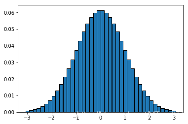
sample_nums = 1000 #采样次数
samples = pd.Series(np.random.choice(x, size=sample_nums, p=p2)) #抽取样本
data = samples.value_counts()
plt.bar(data.index, data.values, barwidth,
edgecolor='black');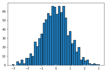
多参数模型中的抽样
假设参数为\(\mathbf{\theta} = (\theta_1, \theta_2)\), \(\theta_1\)为我们感兴趣的参数, 不一定是1维的.
方法1: 由联合后验分布\(\pi(\theta_1, \theta_2|\mathbf{x})\)对\(\theta_2\)积分, 获得\(\theta_1\)的边际分布
\[ \tag{2} \pi(\theta_1|\mathbf{x}) = \int \pi(\theta_1, \theta_2|\mathbf{x}) \mathrm{d} \theta_2. \]
如果上式的积分有显示表达, 可用传统的贝叶斯方法处理? 但是对于许多实际问题, 上述积分无法或很难得到显示表示.
方法2: 由联合后验分布\(\pi (\theta_1, \theta_2 |\mathbf{x})\)直接抽样, 然后仅考察感兴趣参数的样本, 这种方法当参数的维数较低时是可行的.
方法3: 将联合后验分布\(\pi(\theta_1, \theta_2|\mathbf{x})\)进行分解, 写成\(\pi(\theta_2|\mathbf{x}) \times \pi(\theta_1|\theta_2, \mathbf{x})\),这时可将\(\pi(\theta_1|\mathbf{x})\)表示成下面的积分形式
\[ \tag{3} \pi(\theta_1 | \mathbf{x}) = \int \pi(\theta_1 | \theta_2, \mathbf{x}) \pi (\theta_2|\mathbf{x})\mathrm{d}\theta_2, \]
可以解释成\(\pi(\theta_1|\theta_2, \mathbf{x})\)的加权平均\(E^{\theta_2|\mathbf{x}}[\pi(\theta_1|\theta_2, \mathbf{x})]\), 权函数维边际后验分布\(\pi(\theta_2|\mathbf{x})\). 显然这要求\(\pi(\theta_2|\mathbf{x})\)是易得的.
具体步骤如下:
- 从边际后验分布\(\pi(\theta_2, \mathbf{x})\)抽取\(\theta_2\);
- 给定上面已经抽得的\(\theta_2\), 从条件后验分布\(\pi(\theta_1|\theta_2, \mathbf{x})\)中抽取\(\theta_1\).
从书上抄一个例子, 下面是20位选手的马拉松比赛的成绩, 假定它们来自正态分布\(\mathcal{N}(\mu, \sigma^2)\)的样本, 先验分布为:
\[ \tag{4} \pi(\mu, \sigma^2) \propto \frac{1}{\sigma^2}, \]
则其后验分布具有形式
\[ \tag{5} \pi(\mu, \sigma^2|\mathbf{x}) \propto \frac{1}{(\sigma^2)^{n/2+1})} \mathrm{exp}\{{-\frac{1}{\sigma^2}[(n-1)s^2+n(\mu-\bar{x})^2]}\}, \]
其中\(n\)为样本容量, \(\bar{x}=\sum_{i=1}^n x_i / n\)为样本均值, \(s^2 = \sum_{i=1}^n (x_i-\bar{x})^2 / (n-1)\)为样本方差.
x = [
    182, 201, 221, 234, 237, 251, 261, 266, 267, 273,
    286, 291, 292, 296, 296, 296, 326, 352, 359, 365
]
x = pd.Series(x)  #数据
n = len(x)
x_mean = x.mean() #均值
x_variance = x.var() #方差
n, x_mean, x_variance
(20, 277.6, 2454.0421052631577)计算\(\mu\)的边际后验分布
\[ \tag{6} \pi(\mu|\mathbf{x}) \propto [1 + \frac{n(\mu-\bar{x})^2}{(n-1)s^2}]^{-n/2}, \]
它是自由度为n-1, 位置参数为\(\bar{x}\), 刻度参数为\(s^2 / n\)的t分布, 即
\[ \tag{7} \frac{\mu - \bar{x}}{s/\sqrt{n}} |\mathbf{x} \sim t(n-1). \]
samples = stats.t.rvs(n-1, size=1000) # 按照t分布抽取1000个样本
mus = samples * np.sqrt(x_variance / n) + x_mean #转换为均值
the_min, the_max = mus.min(), mus.max()
groups, group_count, barwidth = group_inf(mus, the_min, the_max, group_nums=20)
fig, ax = plt.subplots()
ax.bar(groups, group_count/1000, barwidth, edgecolor='black')
ax.plot(groups, group_count/1000, color='red')
ax.set_xlabel(r'$\mu$')
ax.set_ylabel('Density');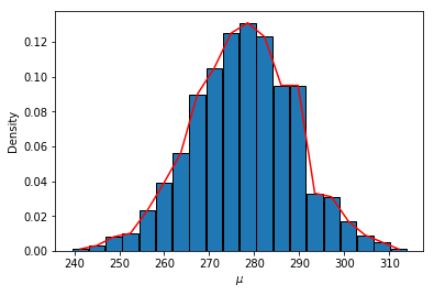
接下来, 通过联合后验分布的分解, 利用第三种方法进行贝叶斯分析,
\[ \tag{8} \pi(\mu, \sigma^2 | \mathbf{x}) = \pi ( \sigma^2 | \mathbf{x}) \times \pi (\mu | \sigma^2, \mathbf{x}). \]
容易得到
\[ \tag{9} \pi (\mu | \sigma^2, \mathbf{x}) = \mathcal{N}(\bar{x}, \sigma^2 / n). \]
根据(5)式可以得到
\[ \tag{10} \pi(\sigma^2 | \mathbf{x}) \propto (\sigma^2)^{-(\frac{n-1}{2}+1)} \mathrm{exp}(-\frac{(n-1)s^2}{2\sigma^2}), \]
故它是倒卡方分布的核, 整理后得到
\[ \tag{11} \frac{(n-1)s^2}{\sigma^2} | \mathbf{x} \sim \chi^2 (n+3). \]
samples_sigma = stats.chi2.rvs(n+3, size=1000) #从自由度n-1的卡方分布中抽取Y, 并解出对于的sigma^2
sigma2s = (n-1) * x_variance / samples_sigma
mus = stats.norm.rvs(x_mean, scale=np.sqrt(sigma2s / n)) #给定方差, 从正态分布中抽取均值, scale参数相当于标准差
the_min, the_max = mus.min(), mus.max()
groups, group_count, barwidth = group_inf(mus, the_min, the_max, group_nums=20)
fig, ax = plt.subplots()
ax.bar(groups, group_count/1000, barwidth, edgecolor='black')
ax.plot(groups, group_count/1000, color='red')
ax.set_xlabel(r'$\mu$')
ax.set_ylabel('Density');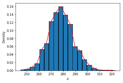
Gibbs 抽样
定义\(\mathbf{\theta} = (\theta_1, \theta_2, \ldots, \theta_p)\), 在Gibb抽样中, 称
\[ \tag{12} \pi (\theta_j | \theta_{-j},\mathbf{x}) = \frac{\pi (\theta|\mathbf{x})}{\int \pi(\mathbf{\theta}|\mathbf{x}) \mathrm{d}\theta_j}, \quad j = 1, 2, \ldots, p \]
为\(\theta_j\)的满条件分布, 其中\(\theta_{-j} = (\theta_1, \ldots, \theta_{j-1}, \theta_{j+1}, \ldots, \theta_p)\). 假设这\(p\)个满条件分布均可容易抽样, 则Gibbs抽样可以如下进行:
- 给定参数的初始值: \(\theta_1^{(0)}, \theta_2^{(0)}, \cdots, \theta_p^{(0)}\);
- 对\(t=0, 1, 2,\cdots,\)进行下面的迭代更新:
- 从分布\(\pi(\theta_1| \theta_2^{(t)}, \cdots, \theta_p^{(t)}, \mathbf{x})\)中产生\(\theta_1^{(t+1)}\);
- 从分布\(\pi(\theta_2| \theta_2^{(t+1)}, \theta_3^{(t)}, \cdots, \theta_p^{(t)}, \mathbf{x})\)中产生\(\theta_2^{(t+1)}\);
- ……
- 从分布\(\pi(\theta_p| \theta_1^{(t+1)}, \theta_2^{(t+1)}, \cdots, \theta_{p-1}^{(t+1)}, \mathbf{x})\)中产生\(\theta_p^{(t+1)}\);
例子1
回到马拉松的例子, 由(5)式得到\(\sigma^2\)的条件后验分布为:
\[ \tag{13} \pi(\sigma^2 | \mu, \mathbf{x}) = \frac{\pi(\mu, \sigma^2 | \mathbf{x})}{\pi (\mu|\mathbf{x})} \propto \frac{1}{(\sigma^2)^{[n/2+1]}} \mathrm{exp} (-\frac{A}{2 \sigma^2}), \]
即
\[ \tag{14} \frac{A}{\sigma^2} | \mathbf{x} \sim \chi^2(n+4), \]
其中\(A=(n-1)s^2+n(\mu - \bar{x})^2\).
另外, \(\mu\)的条件后验分布以及由(9)式得到了.
def garnish(**init):
    def decorater(func):
        def wrapper(*args, **kwargs):
            kwargs.update(init)
            result = func(*args, **kwargs)
            return result
        wrapper.__name__ = func.__name__
        wrapper.__doc__ = func.__doc__
        return wrapper
    return decorater

@garnish(n=n, x_mean=x_mean, x_variance=x_variance)
def A(mu, n, x_mean, x_variance):
    return (n-1) * x_variance + n * (mu - x_mean) ** 2
mu, sigma2 = x_mean/2, x_variance / n #初始化 实际上方差的初始化没有意义
t = 1500
process_mu = [mu]
process_sigma2 = [sigma2]
for i in range(t):
temp = stats.chi2.rvs(n+4)
sigma2 = A(mu) / temp
mu = stats.norm.rvs(x_mean, scale=np.sqrt(sigma2 / n))
process_mu.append(mu)
process_sigma2.append(sigma2)
fig, ax = plt.subplots()
ax.plot(np.arange(1, t+1), process_mu[1:])
ax.set_xlabel("times")
ax.set_ylabel(r"$\mu$");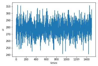
例子2
当Gibbs抽样中的满条件后验分布不易抽样的时候, 我们可以通过引入辅助变量(实际上还有别的方法, 这里就记一下这一种), 拆分后验分布中复杂的项, 使得辅助变量与模型参数的满条件后验分布变得容易抽样.
在基因连锁模型中, 某个实验有5个可能的结果, 出现的概率分别为:
\[ \tag{15} (\frac{\theta}{4} + \frac{1}{8}), \frac{\theta}{4}, \frac{\eta}{4}, (\frac{\eta}{4}+\frac{3}{8}), \frac{1}{2}(1-\theta-\eta), \]
其中\(0\le \theta, \eta \le 1\)为位置参数. 现在进行独立的试验, 出现各结果的次数为\(\mathbf{y} = (y_1,\ldots, y_5) = (14, 1, 1, 1, 5)\).
ys = (14, 1, 1, 1, 5)若取\((\theta, \eta)\)的先验为无信息平坦先验
\[ \tag{16} \pi(\theta, \eta) \propto 1, \]
则\((\theta, \eta)\)的后验分布为
\[ \tag{17} \pi(\theta, \eta|\mathbf{y}) \propto (2\theta + 1)^{y_1} \theta^{y_2} \eta^{y_3} (2\eta + 3)^{y_4} ( 1-\theta-\eta)^{y_5}. \]
上面的分布不容易抽样, 可以引入辅助变量将概率\(p_1, p_4\)拆分.
\[ \tag{18} Y_1 = Z_1 + (Y_1 - Z_1) \\ Y_4 = Z_2 + (Y_4 - Z_2), \]
则\((Z_1, Y_1 - Z_1, Y_2, Y_3, Z_2, Y_4-Z_2, Y_5)\)服从多项分布
\[ \tag{19} M[22; \frac{\theta}{4}, \frac{1}{8}, \frac{\theta}{4}, \frac{\eta}{4}, \frac{\eta}{4}, \frac{3}{8}, \frac{1}{2}(1-\theta-\eta)], \]
其中\(M(n;p_1,\ldots, p_k)\)表示试验次数为\(n\), 参数为\(p_1, \ldots, p_k)\)的多项分布, \(\mathbf{Z} = (Z_1, Z_2)\)是不可观测的, 可看作缺失数据, 在贝叶斯分析红可以看作参数.
在无信息平坦先验下, \((\theta, \eta, Z_1, Z_2)\)的联合后验分布为
\[ \tag{20} \pi (\theta, \eta, Z_1, Z_2| \mathbf{y}) \propto (\frac{\theta}{4})^{Z_1+y_2} (\frac{1}{8})^{y_1 - Z_1} ( \frac{\eta}{4})^{y_3+Z_2} (\frac{3}{8})^{y_4-Z_2} (\frac{1-\theta-\eta}{2})^{y_5}. \]
则
\[ \tag{21} \begin{array}{ll} \pi (\theta| \eta, Z_1, Z_2, \mathbf{y}) & \propto \theta^{Z_1 + y_2} (1 - \eta - \theta)^{y_5} \\ & \propto (\frac{\theta}{1-\eta}^{(Z_1 + y_2 + 1) - 1} (1 - \frac{\theta}{1-\eta})^{(y_5 + 1) - 1}, \end{array} \]
所以
\[ \tag{22} \frac{\theta}{1-\eta} | \eta, Z_1, Z_2, \mathbf{y} \sim Beta(Z_1 + y_2 +1, y_5+1), \theta \in [0, 1 - \eta], \]
同理
\[ \tag{23} \frac{\eta}{1-\theta} | \theta, Z_1, Z_2, \mathbf{y} \sim Beta(Z_2+y_3+1, y_5+1), \eta \in [0, 1-\theta ]. \]
另外:
\[ \tag{24} \begin{array}{ll} \pi (Z_1 | \theta, \eta, Z_2, \mathbf{y}) & \propto (\frac{\theta}{4})^{Z_1} (\frac{1}{8})^{y_1-Z_1} \\ & \propto (\frac{2\theta}{2\theta+1})^{Z_1} (\frac{1}{2\theta+1})^{y_1-Z_1}, \end{array} \]
其中\(b\)表二项分布, 注意, 为什么次数是\(y_1\), 这是根据我们的对\(Z_1\)的构造得来的.
从而
\[ \tag{25} Z_1 | \theta, \eta, Z_2, \mathbf{y} \sim b(y_1, \frac{2\theta}{2\theta+1}), \\ Z_2 | \theta, \eta, Z_1, \mathbf{y} \sim b (y_2, \frac{2\eta}{2\eta+3}). \]
theta, eta, z1, z2 = (0.1, 0.8, 7, 0.1) #初始化参数
t = 5000
process_theta = [eta]
process_eta =  [theta]
for i in range(t):
    temp = stats.beta.rvs(z1 + ys[1] + 1, ys[4] + 1) #采样并更新theta
    theta = (1 - eta) * temp
    temp = stats.beta.rvs(z2 + ys[2] + 1, ys[4] + 1) #采样并更新eta
    eta = (1 - theta) * temp
    z1 = stats.binom.rvs(ys[0], 2 * theta / (2 * theta + 1)) #采样并更新z1
    z2 = stats.binom.rvs(ys[3], 2 * eta / (2 * eta + 3)) #采样并更新z2
    process_theta.append(theta)
    process_eta.append(eta)
fig, ax = plt.subplots(1, 2)
ax[0].plot(np.arange(t+1), process_theta)
ax[1].plot(np.arange(t+1), process_eta)
ax[0].set_xlabel('t')
ax[1].set_xlabel('t')
ax[0].set_ylabel(r'$\theta$')
ax[1].set_ylabel(r'$\eta$');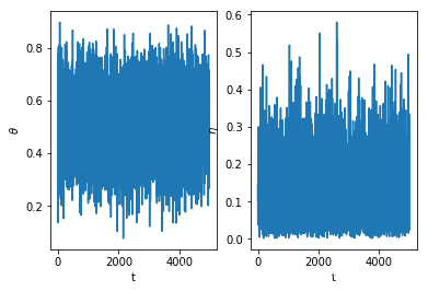
"""
这部分计算后验均值, 每一步的
"""
theta_sum = np.cumsum(process_theta)
eta_sum = np.cumsum(process_eta)
theta_mean = theta_sum / np.arange(1, len(theta_sum)+1)
eta_mean = eta_sum / np.arange(1, len(eta_sum)+1)
fig, ax = plt.subplots(1, 2)
ax[0].plot(np.arange(t+1), theta_mean)
ax[1].plot(np.arange(t+1), eta_mean)
ax[0].set_xlabel('t')
ax[1].set_xlabel('t')
ax[0].set_ylabel(r'$\theta$')
ax[1].set_ylabel(r'$\eta$')
plt.tight_layout();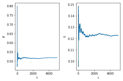
fig, ax = plt.subplots()
start = int(t / 10)
ax.scatter(process_theta[start:], process_eta[start:]) #密集恐惧症患者不要将点空心化, 有点冷
ax.set_xlabel(r'$\theta$')
ax.set_ylabel(r'$\eta$');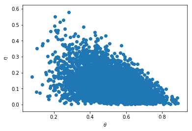
Metropolis-Hastings算法
Metropolis-Hastings算法(MH算法)是一类最为常用的MCMC方法, 它先由Metropolis等提出, 后由Hastings进行推广, 包括特殊情况Gibbs抽样, 及另外三个特殊的MH抽样法: Metropolis抽样, 独立性抽样, 随机游动Metropolis抽样等. MCMC方法的精髓是构造合适的马氏链, 使其平稳分布就是待抽样的目标分布. 在贝叶斯分析中此目标分布就是后验分布\(\pi (\mathbf{\theta}| \mathbf{x})\). 因此MH算法的主要任务是产生满足上述要求的马氏链\(\{\theta^{(t)}, t= 0, 1, 2, \ldots\}\), 即在给定状态\(\theta^{(t)}\)下, 产生下一个状态\(\theta^{(t+1)}\). 所有MH算法的构造框架如下:
- 构造合适的简易分布\(q(\cdot | \theta^{(t)})\);
- 从\(q(\cdot|\theta^{(t)})\)产生候选点\(\theta'\);
- 按一定的接受概率形成的法则取判断是否接受\(\theta'\). 若\(\theta'\)被接受, 则令\(\theta^{(t+1)}=\theta'\), 否则\(\theta^{(t+1)} = \theta^{(t)}\).
MH抽样方法通过如下方式产生马氏链\(\{\theta^{(t)}, t=0,1,2,\ldots\}\)
- 构造合适的建议分布\(q(\cdot| \theta^{(t)})\);
- 从某个分布g中产生\(\theta^{(0)}\)(通常直接给定);
- 重复下面过程直至马氏链达到平稳状态
- 从\(q(\cdot|\theta^{(t)})\)中产生候选点\(\theta'\);
- 从均匀分布\(U(0, 1)\)中产生U;
- 判断: 若
\[ U \le r(\theta^{(t)}, \theta') := \frac{\pi(\theta'|\mathbf{x})q(\theta^{(t)}|\theta')}{\pi(\theta^{(t)}|\mathbf{x})q(\theta'|\theta^{(t)})}, \]
则接受\(\theta'\), 并令\(\theta^{(t+1)} = \theta'\), 否则\(\theta^{(t+1)} = \theta^{(t)}\); - 增加t, 进入下一个循环
Metropolis抽样
Metropolis 抽样是MH算法中的一种特殊抽样方法, 其中的建议分布\(q(\cdot|\theta^{(t)}\)是对称的, 即满足
\[ \tag{26} q(X|Y) = q(Y|X), \]
相应的接受概率变为
\[ \tag{27} \alpha(\theta^{(t)}, \theta') = \min \{1, \frac{\pi( \theta'|\mathbf{x})}{\pi (\theta^{(t)}|\mathbf{x})} \}. \]
随机游动Metropolis抽样
随机游动Metropolis抽样是Metropolis抽样的一个特例,其中对称的建议分布为
\[ \tag{28} q(Y|X) = q(|X-Y|). \]
实际使用时可先从\(q(\cdot)\)中产生一个增量\(Z\), 然后取候选点为\(\theta' = \theta^{(t)}+Z\). 例如从分布\(\mathcal{N}(\theta^{(t)}, \sigma^2)\)中产生的候选点\(\theta'\)克表示为\(\theta' = \theta^{(t)} + \sigma Z\).
独立性抽样法
独立性抽样法也是MH抽样法的特殊情况, 其简易分布不依赖于链前面的值, 即\(q(\cdot| \theta^{(t)}) = q(\cdot)\), 这时的接受概率为
\[ \tag{29} \alpha(\theta^{(t)}, \theta') = \min \{1, \frac{\pi(\theta'|\mathbf{x}) q(\theta^{(t)})}{\pi (\theta^{(t)}| \mathbf{x}) q(\theta')} \}. \]
逐分量MH算法
当目标分布是多维时, 用MH算法进行整体更新往往比较困难, 转而对其分量逐个更新, 这就是所谓的逐分量MH算法的思想, 分量的更新通过满条件分布的抽样来完成,故这种方法又称为Metropolis中的Gibbs算法. 仍用后验分布\(\pi(\theta_1, \cdots, \theta_p|\mathbf{x})\)为目标分布来进行叙述. 记\(\theta = (\theta_1, \cdots, \theta_p)\), \(\theta_{-i} = (\theta_1, \cdots, \theta_{i-1}, \theta_{i+1}, \cdots, \theta_p)\), 则
\[ \tag{30} \theta^{(t)} = (\theta_1^{(t)}, \cdots, \theta_p^{(t)}), \\ \theta^{(t)}_{-i} = (\theta_1^{(t)}, \cdots, \theta_{i-1}^{(t)}, \theta_{i+1}^{(t)}, \cdots, \theta_p^{(t)}). \]
它们分别表示在第t步链的状态和除第i个分量外其它分量在第t步的状态,\(\pi(\theta_i | \theta_{-i}, \mathbf{x})\)为\(\theta_i\)的满条件分布. 在逐分量的MG算法中从t步的\(\theta^{(t)}\)更新到t+1步的\(\theta^{(t+1)}\)分p个小步来完成: 对\(i=1, 2, \cdots, p\),
- 选择建议分布\(q_i(\cdot| \theta_i^{(t)} {\theta_{-i}^{(t)}}^*)\), 其中
\[ {\theta_{-i}^{(t)}}^* = (\theta_1^{(t+1)}, \cdots, \theta_{i-1}^{(t+1)}, \theta_{t+1}^{(t)}, \cdots, \theta_p^{(t)}). \] - 从建议分布\(q_i(\cdot | \theta_i^{(t)}, {\theta_{-i}^{(t)}}^*)\)中产生候选点\(\theta_i'\),并以概率
\[ \tag{31} \alpha (\theta_i^{(t)}, {\theta_{-i}^{(t)}}^*, \theta_i') = \min \big\{ 1, \frac{\pi ( \theta_i'| {\theta_{-i}^{(t)}}^*, \mathbf{x}) q_i(\theta_i^{(t)} | \theta_i^{'}, {\theta_{-i}^{(t)}}^*)} {\pi ( \theta_i^{(t)} | {\theta_{-i}^{(t)}}^*, \mathbf{x}) q_i (\theta_i' | \theta_i^{(t)}, {\theta_{-i}^{(t)}}^*)} \big\} \]
接受\(\theta'_i\).
可见, Gibbs抽样是一种逐分量的MH抽样方法, 其建议分布选为满条件分布\(\pi (\cdot | {\theta_{-i}^{(t)}}^*)\).
一个例子
考察54位老年人的智力测试成绩, 数据如下
x = (
    9, 13, 6, 8, 10,
    4, 14, 8, 11, 7,
    9, 7, 5, 14, 13,
    16, 10, 12, 11, 14,
    15, 18, 7, 16, 9,
    9, 11, 13, 15, 13,
    10, 11, 6, 17, 14,
    19, 9, 11, 14, 10,
    16, 10, 16, 14, 13,
    13, 9, 15, 10, 11,
    12, 4, 14, 20
)

y = [1] * 14 + [0] * 40
df = pd.DataFrame({'x':x, 'y':y}, index=np.arange(1, 55))
df| x | y | |
|---|---|---|
| 1 | 9 | 1 |
| 2 | 13 | 1 |
| 3 | 6 | 1 |
| 4 | 8 | 1 |
| 5 | 10 | 1 |
| 6 | 4 | 1 |
| 7 | 14 | 1 |
| 8 | 8 | 1 |
| 9 | 11 | 1 |
| 10 | 7 | 1 |
| 11 | 9 | 1 |
| 12 | 7 | 1 |
| 13 | 5 | 1 |
| 14 | 14 | 1 |
| 15 | 13 | 0 |
| 16 | 16 | 0 |
| 17 | 10 | 0 |
| 18 | 12 | 0 |
| 19 | 11 | 0 |
| 20 | 14 | 0 |
| 21 | 15 | 0 |
| 22 | 18 | 0 |
| 23 | 7 | 0 |
| 24 | 16 | 0 |
| 25 | 9 | 0 |
| 26 | 9 | 0 |
| 27 | 11 | 0 |
| 28 | 13 | 0 |
| 29 | 15 | 0 |
| 30 | 13 | 0 |
| 31 | 10 | 0 |
| 32 | 11 | 0 |
| 33 | 6 | 0 |
| 34 | 17 | 0 |
| 35 | 14 | 0 |
| 36 | 19 | 0 |
| 37 | 9 | 0 |
| 38 | 11 | 0 |
| 39 | 14 | 0 |
| 40 | 10 | 0 |
| 41 | 16 | 0 |
| 42 | 10 | 0 |
| 43 | 16 | 0 |
| 44 | 14 | 0 |
| 45 | 13 | 0 |
| 46 | 13 | 0 |
| 47 | 9 | 0 |
| 48 | 15 | 0 |
| 49 | 10 | 0 |
| 50 | 11 | 0 |
| 51 | 12 | 0 |
| 52 | 4 | 0 |
| 53 | 14 | 0 |
| 54 | 20 | 0 |
其中\(x_i, y_i\)分别第i个人的智力水平(为等级分,0-20分)和是否患有老年痴呆症(1为是, 0为否). 研究的兴趣在于发现老年痴呆症. 采用logistic模型来刻画上面的数据:
\[ \tag{32} y_i \sim b(1, \theta_i), \log ( \frac{\theta_i}{1-\theta_i}) = \beta_0 + \beta_1 x_i, \: i = 1, 2, \ldots, 54. \]
\((\beta_0, \beta_1)\)的先验分布为独立的正态分布:
\[ \tag{33} \beta_j = \mathcal{N} (\mu_j, \sigma_j^2), \: j = 0, 1, \]
其中\(\mu_j=0\), \(\sigma^2_j\)设得很大, 表示接近无信息先验分布. 由此我们可以得到\((\beta_0, \beta_1)\)的后验分布
\[ \tag{34} \begin{array}{ll} \pi(\beta_0, \beta_1|y) & \propto \pi (\beta_0, \beta_1) p (y | \beta_0, \beta_1) \\ & \propto \exp \big \{ -\frac{(\beta_0 - \mu_0)^2}{2\sigma_0^2}-\frac{(\beta_1 - \mu_1)^2}{2\sigma_1^2} \big \} \\ & \quad \times \prod_{i=1}^n (\frac{e^{\beta_0+\beta_1 x_i}}{1+e^{\beta_0+\beta_1x_i}})^{y_i} (\frac{1}{1+e^{\beta_0+\beta_1 x_i}})^{1-y_i} \end{array} \]
随机游动抽样
第t步的建议分布取为
\[ \beta_j^{(t)} \sim \mathcal{N} (\beta_j^{(t-1)}, \tau_j^2), \: j=0, 1, \]
且\((\tau_0, \tau_1)\)取为\((0,10, 0.10)\).
def posterior_random_walk(x, y, beta, mu, sigma2):
    theta = lambda x: np.exp(beta[0] + beta[1] * x) / ( 1 + np.exp(beta[0] + beta[1] * x))
    return np.exp(-(beta[0] - mu[0]) ** 2 / (2 * sigma2[0]) -
                 (beta[1] - mu[1]) ** 2 / (2 * sigma2[1])) * (
                theta(x) ** y * (1 - theta(x)) ** (1 - y)
            ).prod()
def random_walk(x, y, beta0=0., beta1=0.,
                mu=(0., 0.), sigma2=(10000, 10000),
                tau=(0.1, 0.1), times=5000):
    mu = np.array(mu)
    tau = np.array(tau)
    process_0 = [beta0]
    process_1 = [beta1]
    count = 0
    for t in range(times):
        temp = stats.multivariate_normal.rvs(   #采样
                                mean=(beta0, beta1),
                                cov=np.diag((tau[0], tau[1]))
                            )
        alpha = min(1,   #计算接受概率
                    posterior_random_walk(x, y, temp, mu, sigma2) /
                   posterior_random_walk(x, y, (beta0, beta1), mu, sigma2))

        if np.random.rand() < alpha:
            beta0, beta1 = temp
            process_0.append(beta0)
            process_1.append(beta1)
            count += 1
    return process_0, process_1, count / times
process0, process1, acc_rate = random_walk(df['x'], df['y'])n = len(process0)
n, acc_rate #这个拒绝率也太高了点吧(671, 0.134)cum_mean0 = np.cumsum(process0) / np.arange(1, n + 1) #计算遍历均值
cum_mean1 = np.cumsum(process1) / np.arange(1, n + 1)
fig, ax = plt.subplots(2, 2)
for i in range(2):
for j in range(2):
ax[i, j].set_xlabel(r't')
ax[i, j].set_ylabel(r'$\beta^{(t)}_' + str(j) + '$')
ax[0, 0].plot(np.arange(0, n), process0)
ax[0, 1].plot(np.arange(0, n), process1)
ax[1, 0].plot(np.arange(0, n), cum_mean0)
ax[1, 1].plot(np.arange(0, n), cum_mean1)
plt.tight_layout()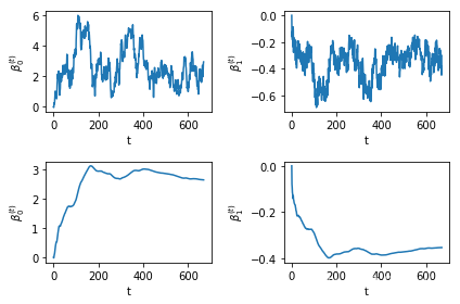
MH抽样 多元正态建议分布
上面的抽样的链的混合效率低下的原因是我们所选取的\(\beta_0, \beta_1\)的建议分布是相互独立的. 解决此问题的一个自然的办法是考虑非独立的建议分布, 且建议分布的相关阵与后验分布的相关阵类似.为此, 我们考虑使用Fisher信息阵(这部分的内容忘了, 不想深究, 就直接套用公式来, 很有可能是错的) \(H(\mathbf{\beta})\), 迭代的建议分布取为
\[ \mathbf{\beta}' \sim \mathcal{N} (\mathbf{\beta}, c_{\beta}^2 [H(\mathbf{\beta})]^{-1}, \]
其中\(c_{\beta}\)为调节参数, 以使算法达到预先设定的接受率. \(\mathbf{\beta} = (\beta_0, \beta_1)\)仍取独立的正态先验, 即\(\mathcal{N}(\mathbf{\mu}_{\beta}, \Sigma_{\beta})\), 其中\(\mathbf{\mu}_{\beta} = (0, 0), \Sigma_{\beta} = \mathrm{diag} \{ \tau_0^2, \tau_1^2\}\). 由(34)知Fisher信息阵为
\[ X^T \mathrm{diag} (h_1, \cdots, h_{54}) X + \Sigma_{\beta}^{-1}, \]
其中\(X = (1_n, \mathbf{x}) \in \mathbb{R}^{n \times 2}\),
\[ h_i = \frac{\exp (\beta_0 + \beta_1 x_i)}{ ( 1 + \exp (\beta_0 + \beta_1 x_i))^2}. \]
此MH算法的抽烟步骤如下:
- 给定\(\mathbf{\beta}\)的初值\(\mathbf{\beta}^{(0)}=(0, 0)\);
- 对于\(t=1, 2, \cdots,\)进行下面的迭代,直到收敛为止, 令\(\mathbf{\beta} = \mathbf{\beta}^{(t-1)}\),
- 计算Fisher信息阵
\[ h_i = \frac{\exp (\beta_0 + \beta_1 x_i)}{ ( 1 + \exp (\beta_0 + \beta_1 x_i))^2}, \\ X^T \mathrm{diag} (h_1, \cdots, h_{54}) X + \Sigma_{\beta}^{-1},\\ S_{\beta} = c_{\beta}^2 [H(\mathbf{\beta})]^{-1}. \] - 从正态建议分布\(\mathcal{N}(\mathbf{\beta}, S_{\beta})\)产生候选点\(\mathbf{\beta}'\).
- 计算接受概率
\[ \tag{35} r(\mathbf{\beta}, \mathbf{\beta}') = \frac{p(\mathbf{y} | \mathbf{\beta}') \varphi(\mathbf{\beta}' | \mathbf{\mu}_{\beta}, \Sigma_{\beta}) \varphi(\mathbf{\beta} | \mathbf{\beta}', S_{\beta'})}{p(\mathbf{y} | \mathbf{\beta}) \varphi(\mathbf{\beta}' | \mathbf{\mu}_{\beta}, \Sigma_{\beta}) \varphi(\mathbf{\beta}' | \mathbf{\beta}, S_{\beta'})} \\ \alpha(\mathbf{\beta}, \mathbf{\beta}') = \min \{1, r(\mathbf{\beta, \beta'})\}. \]
并判断是否接受.
def fisher_matrix(x, beta, inv_Sigma, cbeta=1.):
    """
    计算Fisher信息阵
    """
    extend_x = np.vstack((np.ones_like(x), x))
    extend_x = extend_x.astype(float)
    temp = np.exp(beta[0] + beta[1] * x)
    h = (temp / (1 + temp) ** 2).values
    H = extend_x * h @ extend_x.T + inv_Sigma
    cov = cbeta ** 2 * np.linalg.inv(H)
    return cov
oldbeta: \(\mathbf{\beta}\)
newbeta: \(\mathbf{\beta}'\),
mu: \(\mathbf{\mu}_{\beta}\),
sigma: \(\Sigma_{\beta}\),
cov1: \(S_{\beta}\),
cov2: \(S_{\beta'}\).
def p(x, y, beta):
    temp = np.exp(beta[0] + beta[1] * x)
    theta = temp / (1 + temp)
    theta2 = 1 / (1 + temp)
    return (theta ** y * theta2 ** (1 - y)).prod()

def acc_prop(x, y, oldbeta, newbeta, mu, sigma, covold, covnew):
    """计算接受概率"""
    p1 = p(x, y, oldbeta)
    p2 = p(x, y, newbeta)
    phi1 = stats.multivariate_normal.pdf(oldbeta, mean=mu, cov=sigma)
    phi2 = stats.multivariate_normal.pdf(newbeta, mean=mu, cov=sigma)
    q1 = stats.multivariate_normal.pdf(newbeta, mean=oldbeta, cov=covold)
    q2 = stats.multivariate_normal.pdf(oldbeta, mean=newbeta, cov=covnew)
    r =  p2 * phi2 * q2 / (p1 * phi1 * q1)
    return min(1, r)

def mh_sampling(x, y, beta=(0., 0.), mu=(0., 0.), cbeta=1., sigma=None, times=1000):
    if sigma is None:
        sigma = np.array((35 ** 2, 0.20 ** 2))  #注意到我这里取的 35, 0.20, 而3.5和35是类似的, 但是取1以下就很难弄了
        inv_sigma = np.diag(1 / sigma)
        sigma = np.diag(sigma)
    else:
        inv_sigma = np.linalg.inv(sigma)
    process0 = [beta[0]]
    process1 = [beta[1]]
    count = 0
    for t in range(times):
        covold = fisher_matrix(x, beta, inv_sigma, cbeta=cbeta) #计算Fisher信息阵
        newbeta = stats.multivariate_normal.rvs(mean=beta, cov=covold)  #采样
        covnew = fisher_matrix(x, newbeta, inv_sigma, cbeta=cbeta) #计算新的Fisher信息阵
        alpha = acc_prop(x, y, beta, newbeta, mu, sigma, covold, covnew)#计算接受概率
        if np.random.rand() < alpha:
            beta = newbeta
            process0.append(beta[0])
            process1.append(beta[1])
            count += 1
    return process0, process1, count / times
process0, process1, acc_rate = mh_sampling(df['x'], df['y'], cbeta= 0.5, times=4000)acc_rate0.74n = len(process0)
starts = 0 #从0个往后再开始取平均
cum_mean0 = np.cumsum(process0[starts:]) / np.arange(1, n + 1 - starts) #计算遍历均值
cum_mean1 = np.cumsum(process1[starts:]) / np.arange(1, n + 1 - starts)
fig, ax = plt.subplots(2, 2)
for i in range(2):
for j in range(2):
ax[i, j].set_xlabel(r't')
ax[i, j].set_ylabel(r'$\beta^{(t)}_' + str(j) + '$')
ax[0, 0].plot(np.arange(0, n - starts), process0[starts:])
ax[0, 1].plot(np.arange(0, n - starts), process1[starts:])
ax[1, 0].plot(np.arange(0, n - starts), cum_mean0)
ax[1, 1].plot(np.arange(0, n - starts), cum_mean1)
plt.tight_layout()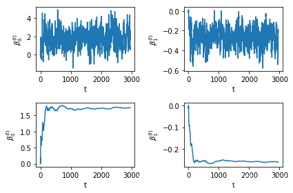
n = len(process0)
starts = 1000  #从1000个往后再开始取平均
cum_mean0 = np.cumsum(process0[starts:]) / np.arange(1, n + 1 - starts) #计算遍历均值
cum_mean1 = np.cumsum(process1[starts:]) / np.arange(1, n + 1 - starts)
fig, ax = plt.subplots(2, 2)
for i in range(2):
    for j in range(2):
        ax[i, j].set_xlabel(r't')
        ax[i, j].set_ylabel(r'$\beta^{(t)}_' + str(j) + '$')
ax[0, 0].plot(np.arange(0, n - starts), process0[starts:])
ax[0, 1].plot(np.arange(0, n - starts), process1[starts:])
ax[1, 0].plot(np.arange(0, n - starts), cum_mean0)
ax[1, 1].plot(np.arange(0, n - starts), cum_mean1)
plt.tight_layout()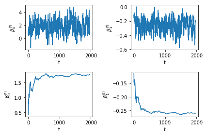
书上没有具体给\(c_{\beta}\)的预设值, 实验发现大的值会导致低的接受率, 另一方面, 如果\(\Sigma_{\beta}\)的选取如果与先前的一致, 结果并不理想, MH对参数如此敏感? 那岂非得有足够的先验才能合理地调整数据? 再经过一些实验发现, \(\Sigma_{\beta}\)取大一点就可以, 达到一定程度就稳定了, 这样看来就很不错了.
逐分量MH抽样
在MH算法中, 按二个分量\(\beta_0\)和\(\beta_1\)进行逐个更新, 这仅设计一维分布的抽样, 且不需要考虑参数的调节. \(\beta_0\)和\(\beta_1\)各自的建议分布用随机游动抽样中的分布,即
\[ \tag{36} \beta_j' = \mathcal{N}(\beta_j, \tau_j^2), j = 0, 1, \]
算法如下:
- 给定\(\mathbf{\beta}\)的初值\(\beta^{(0)} = (0, 0)\);
- 对于\(t=1,2, \cdots\), 进行下面的迭代, 直到收敛为止. 令\(\mathbf{\beta} = \mathbf{\beta}^{(t-1)}\)
- 从正态建议分布\(\mathcal{N} (\beta_0, \tau_0^2)\)产生候选点\(\beta_0'\),
- 令\(\mathbf{\beta}' = (\beta_0', \beta_1^{(t-1)})\), 计算接受概率
\[ \alpha_0 (\mathbf{\beta}, \mathbf{\beta}') = \min \{1, \frac{p(\mathbf{y}| \beta_0', \beta_1), \varphi(\beta_0'| \beta_0, \tau_0^2)}{p(\mathbf{y}| \beta_0, \beta_1), \varphi(\beta_0| \beta_0', \tau_0^2)}\}, \]
并判断是否接受\(\beta_0'\). - 从正态建议分布\(\mathcal{N}(\beta_1, \tau_1^2)\)中产生候选点\(\beta_1'\),
- 令\(\mathbf{\beta}' = (\beta_0^{(t)}, \beta_1'\), 计算接受概率
\[ \alpha_1 (\mathbf{\beta}, \mathbf{\beta}') = \min \{1, \frac{p(\mathbf{y}| \beta_0, \beta_1'), \varphi(\beta_1'| \beta_1, \tau_1^2)}{p(\mathbf{y}| \beta_0, \beta_1), \varphi(\beta_1| \beta_1', \tau_1^2)}\}. \]
并判断是否接受\(\beta_1'\)
def alpha_each_mh1(x, y, oldbeta0, newbeta0, beta1, tau=1.75):
    p1 = p(x, y, (newbeta0, beta1))
    p2 = p(x, y, (oldbeta0, beta1))
    phi1 = stats.norm.pdf(newbeta0, loc=oldbeta0, scale=tau)
    phi2 = stats.norm.pdf(oldbeta0, loc=newbeta0, scale=tau)
    r = p1 * phi1 / (p2 * phi2)
    return min(1, r)


def alpha_each_mh2(x, y, beta0, oldbeta1, newbeta1, tau=0.20):
    p1 = p(x, y, (beta0, newbeta1))
    p2 = p(x, y, (beta0, oldbeta1))
    phi1 = stats.norm.pdf(newbeta1, loc=oldbeta1, scale=tau)
    phi2 = stats.norm.pdf(oldbeta1, loc=newbeta1, scale=tau)
    r = p1 * phi1 / (p2 * phi2)
    return min(1, r)

def mh_each(x, y, beta=[0., 0.], tau=(1.75, 0.20), times=3000):
    process0 = [beta[0]]
    process1 = [beta[1]]
    for t in range(times):
        newbeta0 = stats.norm.rvs(beta[0], tau[0])
        alpha = alpha_each_mh1(x, y, beta[0], newbeta0, beta[1], tau[0])
        if np.random.rand() < alpha:
            beta[0] = newbeta0
            process0.append(beta[0])
        newbeta1 = stats.norm.rvs(beta[1], tau[0])
        alpha = alpha_each_mh2(x, y, beta[0], beta[1], newbeta1, tau[1])
        if np.random.rand() < alpha:
            beta[1] = newbeta1
            process1.append(beta[1])
    return process0, process1
process0, process1 = mh_each(df['x'], df['y'])n1 = len(process0)
n2 = len(process1)
starts = 0 #从0个往后再开始取平均
cum_mean0 = np.cumsum(process0[starts:]) / np.arange(1, n1 + 1 - starts) #计算遍历均值
cum_mean1 = np.cumsum(process1[starts:]) / np.arange(1, n2 + 1 - starts)
fig, ax = plt.subplots(2, 2)
for i in range(2):
for j in range(2):
ax[i, j].set_xlabel(r't')
ax[i, j].set_ylabel(r'$\beta^{(t)}_' + str(j) + '$')
ax[0, 0].plot(np.arange(0, n1 - starts), process0[starts:])
ax[0, 1].plot(np.arange(0, n2 - starts), process1[starts:])
ax[1, 0].plot(np.arange(0, n1 - starts), cum_mean0)
ax[1, 1].plot(np.arange(0, n2 - starts), cum_mean1)
plt.tight_layout()
最后记一笔
这里提到, 为了保证马氏链的平稳分布存在, 需要满足:
\[ \tag{A.1} p(x'|x)p(x) = p(x|x')p(x'). \]
等价于:
\[ \tag{A.2} \frac{p(x'|x)}{p(x|x')} = \frac{p(x')}{p(x)}. \]
当建议分布为\(q(x'|x)\), 而接受概率为\(a(x',x)\)的时候, 我们有
\[ p(x'|x)=q(x'|x)a(x',x), \]
所以需要满足:
\[ \tag{A.3} \frac{a(x', x)}{a(x,x')} = \frac{p(x')q(x|x')}{p(x)q(x'|x)}, \]
而当接受概率定义为
\[ a(x', x) = \min \big(1, \frac{p(x')q(x|x')}{p(x)q(x'|x)} \big), \]
的时候, (A.3)就成立了, 因为一个为1另一个为后面的部分.
我在看书的时候有这样一个问题:
\[ \tag{A.4} p(x')q(x|x') = p(x')\frac{p(x, x')}{p(x')} = p(x, x'), \]
\[ \tag{A.5} p(x)q(x'|x) = p(x)\frac{p(x, x')}{p(x)} = p(x, x'). \]
那么接受概率不就恒为1了? 实际上, 这里我犯了一个误区,注意到, (A.4), (A.5)单独拿出来都是对的, 但是不能合起来看, 因为合起来看的话就默认了一个条件:
\[ p(x|x')=q(x|x'), p(x'|x)=q(x'|x), \]
显然这是不合理的.