摘自:
https://www2.eecs.berkeley.edu/Research/Projects/CS/vision/classes/cs294_f99/notes/lec7/lec7.htm
Gibbs Distribution
Proving Gibbs Distribution Implies Markov Random Field
Trivial because of exponential
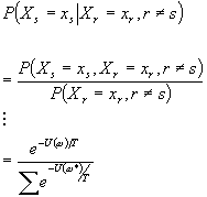
Look at the handout given in class for a detailed proof.
In summary, at the end of the day, sites without s cancel.
Back to the Image Segmentation Problem
Our image model
 |
|||
|
|||
line process l not observed
Goal
- Given observed image g, find a probability distribution of true image f, and the line process l.
The line process estimate solves the image segmentation problem.
The true image estimate solves the image restoration problem.
Both problems are simultaneously solved!
- Note: only works for piecewise smoothe images Þ no textures
Our model assumes:

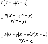
Our solution:
|

 |
Interesting term:
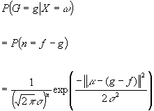
Where we assume every pixel has independent noise h ~ N ( m , s )
e.g. Poisson process noise in CCDs
Result:
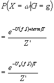
is the posterior probability of a particular f, l given g. Note this is also a Gibbs distribution!
MAP (maximum a posteriori) Estimate
If you insist on a single answer then return f*, l* that maximizes

or equivalently, minimizes the energy function
![]()
Problem: f , l space is very large!!
Solution: Construct samples of f , l in this space with high probablity
Technique: Markov Chain Monte Carlo (MCMC) lets you sample the posterior distribution
Sampling a Distribution
Q: How do we represent a probability distribution with sampling?
A: Create many samples drawn from that distribution and count!
Example:
Q: P(X > 17) = ?
A: Create samples Xi drawn from the distribution of X.
![]()
Count the number of samples greater than 17 and divide by total number of samples.
Generating the Samples
Primitive random number generator X ~ U(0,1).
To create Y ~ U(a,b) use
Y = a + ( b – a ) X
In general we can use the cumulative distribution function
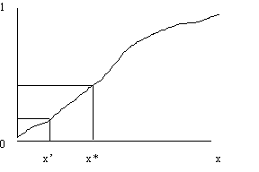
1987 – Stochastic Simulation (Ripley) for generating samples for “standard stuff” in textbooks
Markov Chain Monte Carlo (MCMC) Technique
- Define a suitable Markov Chain whose equilibrium distribution is the desired posterior distribution
- Generate samples from the Markov Chain
Markov Chain Basics
![]()
Example:

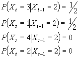
This transition probabilities can be written as a matrix
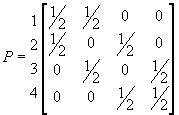
If we write the probability distribution at time t as p(t) then
p(t+1) = p(t)P
For example if the drunk’s walk starts at position 2 we denote
p( t = 0 ) = [0 1 0 0]
p(t) is an evolving probability distribution which is a row vector that sums to one
The equilibrium distribution p(infinity) = p satisfies
pP = p
and is a left eigenvector of P with eigenvalue one.
Finding the Markov Chain Corresponding to the Posterior Distribution
Metropolis Sampler – Rosenberg, Teller, Teller
Heat Bath ( Gibbs Sampler ) – “rapidly mixing” determines convergence rate
Metropolis Sampler
We are given that the posterior distribution is of the form f(x)/Z
1. We have a proposal kernal satisfying K(x,y) = K(y,x)
2. Calculate f(y)
3. Accept transition with probability = min {1, f(y)/f(x) }
4. This eventually converges to the “right thing”
