【Focal Loss】《Focal Loss for Dense Object Detection》

版权声明：本文为博主原创文章，遵循 CC 4.0 BY-SA 版权协议，转载请附上原文出处链接和本声明。

本文链接： https://blog.csdn.net/bryant_meng/article/details/80977517

ICCV-2017

【AI Talking】Focal Loss ICCV2017 现场演讲（Tsung-Yi Lin）

---

---

1 Background and Motivation

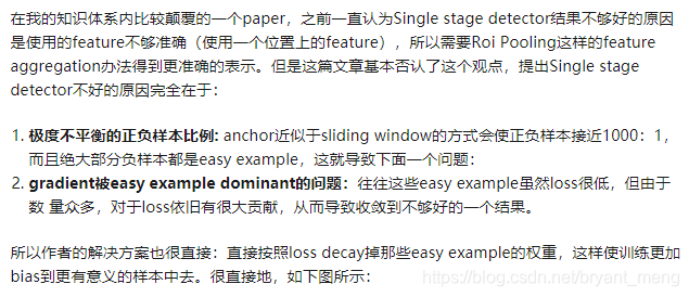
在 COCO 数据集上，two stage 在精度上独占鳌头，one stage 在速度上独领风骚，能否把 one stage 的精度提上去呢？作者发现 class imbalance during training as the main obstacle impeding one-stage detector from achieving state-of-the-art accuracy.

因此，作者对 cross entropy loss 进行了改进，提出 focal loss，降低 easy example loss 的权重（down-weights the loss assigned to well-classified examples），让网络更加注重 hard example loss！

2 Advantages / Contributions / Innovations

identify class imbalance as the primary obstacle preventing one-stage object detectors from surpassing top-performing, two-stage methods.

提出 focal loss，match the speed of previous one-stage detectors while surpassing the accuracy of all existing state-of-the-art two-stage detectors

3 Related Work

• Classic Object Detectors
  • LeCun 的 handwritten digit recognition
  • Viola and Jones 的 face detection
  • HOG for pedestrian detection
  • DPMs for PASCAL VOC
• Two-stage Detectors（R-CNN family）
• One-stage Detectors（OverFeat, SSD, YOLO）
• Class Imbalance（A common solution is to perform some form of hard negative mining that samples hard examples during training or more complex sampling / reweighing schemes.）

4 Method

注意：the focal loss is applied to all ~100k anchors in each sampled image
不像 RPN 中 heuristic sampling 256（eg：>0.7 positive, <0.3 negative, 1:1 train）

4.1 Focal Loss Definition

二分类 cross-entropy（y = 1 or -1）

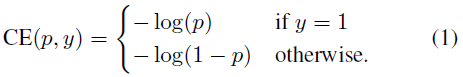
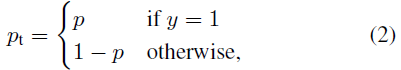
简化一下公式

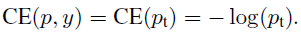
$P_t$ 的定义如下

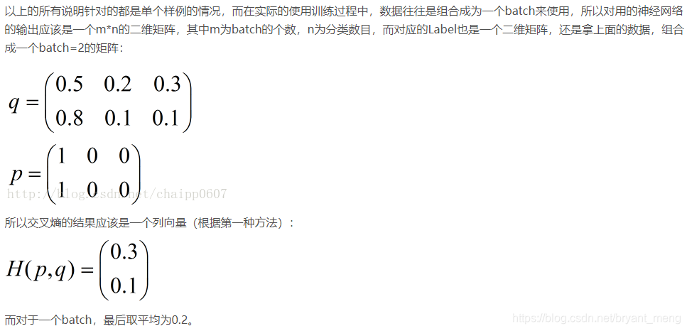
关于 cross entropy 的介绍可以参考 理解交叉熵(cross_entropy)作为损失函数在神经网络中的作用 节选如下：

1）Balanced Cross Entropy
常用的方法是改变正负样本损失的权重，如下所示

$\alpha_t$ 的定义同 $p_t$，具体如下

$\alpha _{t}= \left\{\begin{matrix} \alpha &amp; if \ y=1\\ 1-\alpha &amp; otherwise \end{matrix}\right.$

这种做法能 balance the importance of positive / negative examples, 但是不能 differentiate between easy / hard examples.

2） Focal Loss Definition

具体如下图：

有两个 properties：

• $p_t$ 很小时，unaffected， $p_t$ 很大时，well-classified examples is down-weighted
• $\gamma$ 越大，down-weighted 也相应的变大

具体实现（参考 Focal Loss 的Pytorch 实现以及实验）

3） Class Imbalance and Model Initialization （★★★★★）
引入了 “prior” 的概念，落地的做法就是在 classification subnet 初始化的时候设置了 bias，这样的话 the model’s estimated p for examples of the rare class is low.

这里 rare class 是相对 frequent class 来说的，在二分类中，就是 positive 和 negative 了，class imbalance 的时候，negative 很多，对应着 frequent class.

bias 设置为 $-log((1-\pi)\pi)$， $\pi$ 设置为 0.01，可以看出 bias 是一个很大的负数，不管你是 rare 还是 frequent 感觉强行都拉低到 relu 的响应为 0 区域！能解决 the loss due to the frequent class can dominate total loss and cause instability in early training.

这种做法在哪篇论文中好像看过，不过又记不起来了！

4） Class Imbalance and Two-stage Detectors
first stage 会排除掉大量的无关的 proposals，留下 1000~2000，然后 sampling 到 second stage，eg: positive and negative for 1：3，这里的 1：3 和 4.1 小节的 $\alpha$ 很像！作者的 focal loss 是争对 one-stage 的 classification imbalance 的！

4.2 RetinaNet Detector

ResNet + FPN
与原版 FPN 不同的是

	原版的 FPN	RetinaNet 中的 FPN
level	P2-P6	P3-P7
P6 / P7	P5 max pooling 到 P6，没有 P7	P6 由 P5 3x3 conv，p7 由 P6 3x3 conv

RetinaNet 中没有 P2 for computational reasons，加 P7 improve large object detection

These minor modifications improve speed while maintaining accuracy.

• K object classes, A anchors,

• per spatial position 9 anchor, 原版 FPN，anchor 只有 ratio，scale 归并到 pyramid 去了，这里，在 3 个 ratio {1:2,1:1,2:1} 的基础上，加了3个 scale { $2^0, 2^{1/3}, 2^{2/3}$} ，所以 anchor 的边长从原来的 32~512 （P3-P7，每层 anchor 长 4, $4×2^{level}$）可以到 32~ $512×2^{2/3} = 812.7493386077181$，也就是论文中的 32~813

• positive: iou ≥ 0.5
  negative: iou [0,04)
  [0.4, 0.5) 不参与训练

• inference 的时候，FPN 每层只保留最多 top 1K 的 predictions，0.5 nms for FPN 的 multi-level

5 Experiments

• backbone： resnet-50 、resnet-101
• image size： 600

5.1 Datasets

COCO

• train: trainval 35k（union of 80k images from train and a random 35k subset of images from the 40k image val split）
• val: minival split (the remaining 5k images from val).
• test: test-dev split

1）Balanced Cross Entropy

figure 1， $\alpha = 0.75$ 效果最好

2）Focal Loss

We observe that lower $\alpha$’s are selected for higher $\gamma$’s (as easy negatives are downweighted, less emphasis needs to be placed on the positives).

$\alpha _{t}= \left\{\begin{matrix} \alpha &amp; if \ y=1\\ 1-\alpha &amp; otherwise \end{matrix}\right.$

kaiming的Focal Loss中，为什么当增大γ时，要减小α呢？ - 知乎
https://www.zhihu.com/question/67926031/answer/257937896

3）Analysis of the Focal Loss

累积分布函数(Cumulative Distribution Function)，又叫分布函数，是概率密度函数的积分，能完整描述一个实随机变量X的概率分布。一般以大写CDF标记,，与概率密度函数probability density function（小写pdf）相对（百度百科）。

loss 归一化，从小到大排序，然后累加！

上面图可以简单的理解为，随着样本增加，loss 也在不断的累加

• 左图看出，~20% hardest positive samples account for roughly half of the positive loss（也即，80%累加起来的loss才 0.5 左右），随着 $\gamma$ 的增加， hard positive samples 占的 loss 越多，but the effect is minor
• 右图看出，随着 $\gamma$ 的增加，more weight becomes concentrated on the hard negative examples（FL can effectively discount the effect of easy negatives，focusing all attention on the hard negative examples）

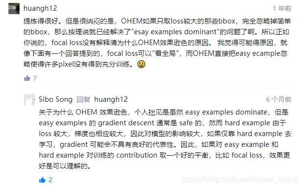
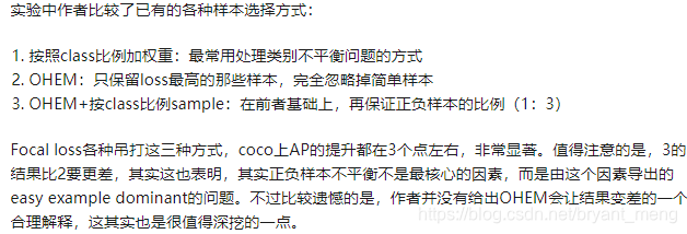
4）Online Hard Example Mining (OHEM)
Like the focal loss, OHEM puts more emphasis on misclassified examples, but unlike FL, OHEM completely discards easy examples.

第一行标注的是 OHEM 论文中的设置（【OHEM】《Training Region-based Object Detectors with Online Hard Example Mining》），Focal Loss 还是很强的！

5）Hinge Loss

focal loss 介于 hinge loss 与 entropy loss 之间

5.2 Model Architecture Design

Anchor Density

ResNet 50

• scale 是 $2^{0}$， $2^{1/4}$， $2^{2/4}$， $2^{3/4}$
• aspect 或者 ratio 是 $\{0.5,1,2\}$，也即 1：2，1：1，2：1！或者只有 1：1

Speed versus Accuracy

下图5个点，对应五个 scale 的输入，400-800 per 100

Comparison to State of the Art

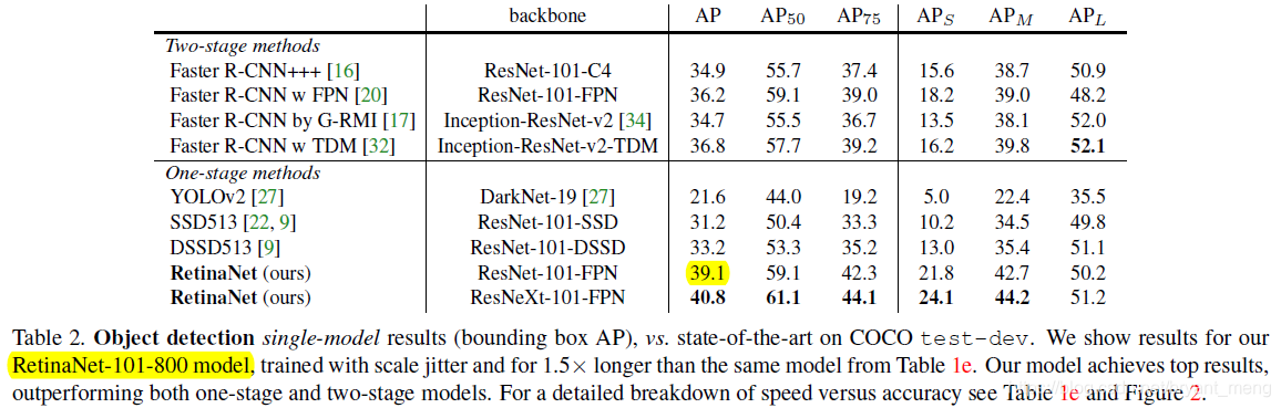
39.1 和 上面的（e）图 37.8 多了 1.3 个点， 因为用了 scale jitter 技术
可以看出，在 one-stage 中的最好结果基础下提升了特别多（33.2-39.1）！也技压 two-stage（36.8-39.1）backbone 换成 ResNeXt 效果进一步提升！

关于scale jittering 的介绍，参考了大牛的讲解，简单来说，就是crop size是固定的，而image size是随机可变的。举例来说，比如把crop size固定在224×224，而image的短边可以按比例缩放到[256, 512]区间的某个随机数值，然后随机偏移裁剪个224×224的图像区域。 （参考 深度卷积神经网络VGG 学习笔记）

6 Conclusion（own）

• 要分清楚正负样本和难易样本的关系
• 要理清 one-stage 的 pipeline，以及和 two-stage 的区别
• 附录中 CE / FL / FL* 求导的推导

7 海纳百川

如何评价Kaiming的Focal Loss for Dense Object Detection？

• Naiyan Wang的回答 - 知乎 https://www.zhihu.com/question/63581984/answer/210832009
  
  

下面是评论区的