文章目录
datawhale_day01
达观杯数据简介
组队学习说明 :
12天的时间实现数据预处理(TF-IDF与word2VEC)->模型实践(朴素贝叶斯,svm与lightgbm)->模型优化
任务路线
数据初始->数据处理->基本模型->实践模型优化->模型优化
任务周期 : 12天
定位人群: 能够熟练使用python,难度系数适中
每个任务周期所需要的时间: 2-3h
任务一:数据初始 时长:1天
1.下载数据,读取数据,观察数据
2.将训练集拆分为训练集和验证集
3.分享自己对数据以及赛题的理解与发现
ps. 电脑爆内存的可以先提取500条数据进行实践
下载数据,读取数据,观察数据
数据包含2个csv文件,
train_set_scv:此数据集用于训练模型,每一行对应一篇文章,文章分别在"字"和""词的级别上做了脱敏处理,共有四列:
第1列: 文章的索引ID
第2列: 文章的正文在"字"的级别上表示,即字符相隔正文(article)
第3列: "词"级别上的表示,即词语相隔正文(word_seg)
第4列: 这篇文章的标注(class)
注: 每一个数字对应一个’字’或’词’,或’标点符号’,'字’的编号与’词’的编号是独立的
test_set.csv: 此数据用于测试数据,同train_set.csv,但不包含class
注:test_set与train_test 中文章id的编号是独立的
# 单行中间变量完全显示
from IPython.core.interactiveshell import InteractiveShell
InteractiveShell.ast_node_interactivity = "all"
import pandas as pd
df_train = pd.read_csv('./new_data/train_set.csv')
df_train.head()
| id | article | word_seg | class | |
|---|---|---|---|---|
| 0 | 0 | 7368 1252069 365865 755561 1044285 129532 1053... | 816903 597526 520477 1179558 1033823 758724 63... | 14 |
| 1 | 1 | 581131 165432 7368 957317 1197553 570900 33659... | 90540 816903 441039 816903 569138 816903 10343... | 3 |
| 2 | 2 | 7368 87936 40494 490286 856005 641588 145611 1... | 816903 1012629 957974 1033823 328210 947200 65... | 12 |
| 3 | 3 | 299237 760651 299237 887082 159592 556634 7489... | 563568 1239563 680125 780219 782805 1033823 19... | 13 |
| 4 | 4 | 7368 7368 7368 865510 7368 396966 995243 37685... | 816903 816903 816903 139132 816903 312320 1103... | 12 |
df_train['article']
0         7368 1252069 365865 755561 1044285 129532 1053...
1         581131 165432 7368 957317 1197553 570900 33659...
2         7368 87936 40494 490286 856005 641588 145611 1...
3         299237 760651 299237 887082 159592 556634 7489...
4         7368 7368 7368 865510 7368 396966 995243 37685...
5         7368 1160791 299237 1238054 569999 1044285 117...
6         893673 7368 836872 674898 231468 856005 105964...
7         1122654 125310 907560 1172361 979583 983951 12...
8         793790 599682 1223643 1030656 569999 178976 45...
9         7368 1120647 360394 79747 1140778 472252 7368 ...
10        734846 28352 316275 979583 1209583 449838 4712...
11        7368 549139 1030656 699820 42898 171803 562056...
12        750606 427848 1068835 544072 493242 953821 887...
13        1016718 486229 7368 569999 862198 7368 7368 81...
14        7368 906650 698148 595261 1274632 1176599 1105...
15        678940 1007781 474675 222667 893126 57871 1044...
16        276639 433631 766202 1209583 865388 318877 359...
17        532914 1101732 316564 868779 905056 1220165 33...
18        979583 1209583 755561 345037 79747 721432 9755...
19        7368 566896 1122688 1044285 473628 153302 3329...
20        324149 417190 979713 570373 527455 856005 2882...
21        7368 422632 56101 1010033 7368 1249227 59456 9...
22        7368 611112 599682 626254 569999 601396 7368 7...
23        330242 788037 40494 1080029 79747 7368 1015617...
24        537848 119827 625647 119827 1044285 427848 101...
25        1220011 206763 837240 678940 641588 206763 314...
26        678940 1007781 172245 314465 721845 326498 758...
27        1252069 569999 1044285 105340 1030191 975571 1...
28        7368 881890 581131 1030656 626254 365865 61111...
29        1209583 906756 755561 345037 79747 106357 9197...
                                ...
102247    951085 265484 1188406 156426 79747 544072 2067...
102248    837240 1188406 1121849 206692 1118173 968221 1...
102249    1091056 1108822 837240 299237 1068835 647476 9...
102250    263884 222667 1010033 760651 394856 1262723 87...
102251    611112 599682 626254 569999 332929 452751 1044...
102252    1077049 1173724 19306 1250888 292474 1044285 3...
102253    430272 326498 159592 453765 239755 332929 9140...
102254    799372 212174 7368 1201957 1158830 544562 7993...
102255    415555 1269463 1201957 1158830 34048 1225691 8...
102256    537848 837240 669302 1111942 856005 670411 178...
102257    849828 550791 42898 1223861 611112 599682 6262...
102258    465701 1122654 1096353 7368 1252114 991700 129...
102259    415555 1269463 332929 452751 768900 285352 759...
102260    380349 707896 678940 1007781 145611 493242 263...
102261    7368 881890 581131 1030656 626254 961786 61111...
102262    1030656 1044285 189578 878425 93932 42898 1262...
102263    649585 559442 1077049 316564 893126 544072 518...
102264    780230 390051 42898 1223861 79747 7368 755289 ...
102265    755561 345037 862965 57871 79747 788037 319764...
102266    1030656 1231714 165432 1231714 365865 1223643 ...
102267    1223643 599682 1030656 1231714 569999 332929 4...
102268    7368 7368 7368 7368 7368 7368 7368 7368 7368 7...
102269    828236 1269463 876762 1220011 206763 1087134 4...
102270    1252069 365865 755561 389346 902663 184021 309...
102271    1122654 850377 1129146 1266092 195449 921820 7...
102272    556634 837240 427848 753262 481583 140141 8560...
102273    611112 599682 626902 569999 178976 452751 1044...
102274    865510 7368 891719 697742 641202 641202 122001...
102275    828236 1269463 474675 180178 1209583 906756 50...
102276    538313 420000 942897 836887 7368 359838 42610 ...
Name: article, Length: 102277, dtype: object
我们可以看到数据共分为’id’,‘article’,‘word_seg’,'class’这四个字段.并且主办方已为我们进行了脱敏,分词,数字化处理
我们对数据进行统计分析:
df_test = pd.read_csv('./new_data/test_set.csv',nrows=5000)
df_test.head()
| id | article | word_seg | |
|---|---|---|---|
| 0 | 0 | 7368 146447 316564 42610 55736 297797 93042 53... | 816903 565958 726082 764656 335008 75094 20282... |
| 1 | 1 | 985531 473628 1044285 1121849 206763 462208 11... | 729468 520477 529032 101368 335130 520477 1113... |
| 2 | 2 | 7368 7368 7368 7368 7368 7368 7368 7368 7368 7... | 816903 816903 816903 816903 816903 816903 8169... |
| 3 | 3 | 529819 1226459 856005 1177293 663773 272235 93... | 231664 1033823 524850 330478 507199 520477 618... |
| 4 | 4 | 42610 1252069 1077049 955883 1125260 1044285 2... | 545370 379223 162767 520477 1194630 1197475 11... |
print(df_train.info(), df_test.info())
<class 'pandas.core.frame.DataFrame'>
RangeIndex: 102277 entries, 0 to 102276
Data columns (total 4 columns):
id          102277 non-null int64
article     102277 non-null object
word_seg    102277 non-null object
class       102277 non-null int64
dtypes: int64(2), object(2)
memory usage: 3.1+ MB
<class 'pandas.core.frame.DataFrame'>
RangeIndex: 5000 entries, 0 to 4999
Data columns (total 3 columns):
id          5000 non-null int64
article     5000 non-null object
word_seg    5000 non-null object
dtypes: int64(1), object(2)
memory usage: 117.3+ KB
None None
print('大家好,我是你们的小可爱~')
查看数据缺失情况
df_train.isnull().any()
id          False
article     False
word_seg    False
class       False
dtype: bool
查看数据分布情况
文本分类共19类,各类别数据均在2000条以上,没有严重的类别不均
df_train['class'].value_counts()
3     8313
13    7907
9     7675
15    7511
18    7066
8     6972
6     6888
14    6740
19    5524
1     5375
12    5326
10    4963
4     3824
11    3571
16    3220
17    3094
7     3038
2     2901
5     2369
Name: class, dtype: int64
划分数据集
数据说明中显示:
'artile'是字级别上的,'word_seg'是词级别的,也就是说举办方已经把单词给我们切好了,不需要自己动手手动分词,已经把单词数字化(脱敏),因此数据划分中x以df_tarin['word_seg']即可
from sklearn.model_selection import train_test_split
X_train, X_test, y_train, y_test = train_test_split(df_train[['word_seg']],
                                                    df_train[['class']],
                                                    test_size = 0.3,
                                                    random_state = 2019)
print (X_train.shape)
print (X_test.shape)
(71593, 1)
(30684, 1)
datawhale day02
【Task2.1】(2天)
学习,使用TF-IDF表示文本
要求:分享学习笔记和代码,【只有代码的等 于没有完成】 https://shimo.im/docs/U2oxcwNa06kitDk5/
参考资料
1)CS 224:https://www.bilibili.com/video/av41393758/?p=2
2)https://github.com/Heitao5200/DGB/blob/master/feature/feature_code/tfidf.py
Tf-IDF 简介
TF; Term-Frequency 词频,指的是给定一个词在改文档中出现的次数
IDF: Inverse Document Frequency 逆文档频率
可以简单的理解成: 一个词语在一篇文章中出现的次数越多,同时在其他的所有文档中出现的次数越少,越能够代表该文章
TF
TF:指的是某一给定的词语在该文档中出现的次数,由于文档的长度不一,防止TF偏向于长文档,需要对其进行归一化处理,一般采取除以文章的总数
TF = 在某一文档中词W出现的次数 / 该文档中所有的词条目数
IDF
如果包含w的文档越少,IDF越大,则说明该词具有很好的类别区分能力
某一特定词语的IDF,可以由总文档数除以包含该词语的文档的数目,再将得到的数除以包含该词语的文档数目,再将得到数取对数得到
IDF= 文档的总和 / (包含该词条的文档树+1)(注:为了防止分母为0,故加1)
TF-IDF
某一特定文件内的高词语频率,以及该词在整个文件集合中的低文件频率,可以产生出高权重的
TF-IDF,因此,TF-IDF倾向于过滤常见的词语,保留重要的词语
例子
一个文档中,总共有1000个词,'中国’出现5次,'体育’出现20次,
总共有100份文档,其中包含’中国’的有30份文档,包含’体育’的有10份文档
中国: TF = 5 / 1000 = 0.005, IDF = log(100 / (30 +1)) = 0.51
体育: TF = 20 /1000 = 0.02, IDF = log(100 / (10 + 1)) = 0.95
中国: TF-IDF = 0.005 * 0.51 = 0.00255
体育; TF-IDF = 0.02 * 0.95 = 0.019
从计算的结果可以看出,‘中国’比’体育’小,如果对文档选择关键词则选择’体育’
code
import pandas as pd
from sklearn.feature_extraction.text import TfidfVectorizer
from sklearn.feature_extraction.text import TfidfTransformer
tfidf_transformer=TfidfTransformer()
import gensim
import pickle
import time
import numpy as np
D:\ProgramData\Anaconda3\lib\site-packages\gensim\utils.py:1209: UserWarning: detected Windows; aliasing chunkize to chunkize_serial
  warnings.warn("detected Windows; aliasing chunkize to chunkize_serial")
# 1.数据预处理
print ('1 数据预处理')

t_start = time.time()

df_train = pd.read_csv('./new_data/train_set.csv',nrows=10000) # 数据大,爆内存,读前10000行
df_test = pd.read_csv('./new_data/test_set.csv',nrows=10000)
df_train.drop(['article'],axis = 1, inplace = True)
df_test.drop(['article'],axis = 1, inplace= True)
f_all = pd.concat(objs = [df_train,df_test],axis = 0)

y_train = (df_train['class'] - 1).values

# Tf-idf
1 数据预处理


D:\ProgramData\Anaconda3\lib\site-packages\ipykernel_launcher.py:10: FutureWarning: Sorting because non-concatenation axis is not aligned. A future version
of pandas will change to not sort by default.

To accept the future behavior, pass 'sort=True'.

To retain the current behavior and silence the warning, pass sort=False

  # Remove the CWD from sys.path while we load stuff.
f_all
| class | id | word_seg | |
|---|---|---|---|
| 0 | 14.0 | 0 | 816903 597526 520477 1179558 1033823 758724 63... |
| 1 | 3.0 | 1 | 90540 816903 441039 816903 569138 816903 10343... |
| 2 | 12.0 | 2 | 816903 1012629 957974 1033823 328210 947200 65... |
| 3 | 13.0 | 3 | 563568 1239563 680125 780219 782805 1033823 19... |
| 4 | 12.0 | 4 | 816903 816903 816903 139132 816903 312320 1103... |
| 5 | 13.0 | 5 | 816903 669476 21577 520477 1004165 4184 616471... |
| 6 | 1.0 | 6 | 277781 816903 1098157 986174 1033823 780491 10... |
| 7 | 10.0 | 7 | 289186 640942 363388 585102 261174 1217680 520... |
| 8 | 10.0 | 8 | 1257015 966562 1054308 599826 811205 520477 28... |
| 9 | 19.0 | 9 | 816903 266069 1226448 1276450 816903 769051 12... |
| 10 | 18.0 | 10 | 398177 792991 282245 431944 507321 572782 5491... |
| 11 | 7.0 | 11 | 816903 824446 426716 1115586 133239 184574 105... |
| 12 | 9.0 | 12 | 699815 422170 1256802 1033823 520259 460600 93... |
| 13 | 4.0 | 13 | 689657 816903 528734 816903 816903 67479 24652... |
| 14 | 17.0 | 14 | 816903 1079905 699727 792255 816903 876555 655... |
| 15 | 9.0 | 15 | 414956 1061507 1145236 520477 701424 1033823 1... |
| 16 | 13.0 | 16 | 970106 821114 460600 1205755 876555 152146 107... |
| 17 | 10.0 | 17 | 745799 1097521 739284 669224 816903 703339 920... |
| 18 | 10.0 | 18 | 282245 769051 1226448 240399 1119534 396212 11... |
| 19 | 14.0 | 19 | 816903 878958 520477 1211157 460600 1070929 80... |
| 20 | 10.0 | 20 | 956848 519291 1033823 31494 454003 327386 5696... |
| 21 | 9.0 | 21 | 816903 727721 329790 816903 1272293 246236 816... |
| 22 | 1.0 | 22 | 816903 340401 966562 102711 599826 1267351 816... |
| 23 | 2.0 | 23 | 713291 135124 1226448 816903 69892 520477 3696... |
| 24 | 13.0 | 24 | 960822 652097 520477 778803 444731 1061507 929... |
| 25 | 1.0 | 25 | 585102 54111 1080587 732777 788023 1033823 120... |
| 26 | 7.0 | 26 | 414956 983449 736182 1032936 355504 1233500 76... |
| 27 | 17.0 | 27 | 1000015 520477 444135 277806 921586 172968 658... |
| 28 | 10.0 | 28 | 816903 386754 553856 340401 966562 340401 5998... |
| 29 | 8.0 | 29 | 1218708 769051 1226448 912033 520477 536257 11... |
| ... | ... | ... | ... |
| 9970 | NaN | 9970 | 557938 1159154 930754 766772 39765 1033823 881... |
| 9971 | NaN | 9971 | 829899 587327 529018 479860 549047 447287 5204... |
| 9972 | NaN | 9972 | 689812 792991 816903 717834 816903 278602 1025... |
| 9973 | NaN | 9973 | 143039 816903 1122752 520477 636415 762897 109... |
| 9974 | NaN | 9974 | 874561 358495 177456 938169 801241 520477 1072... |
| 9975 | NaN | 9975 | 866914 54111 4184 1132352 526298 325497 782716... |
| 9976 | NaN | 9976 | 816903 450633 520477 655201 403305 872389 1100... |
| 9977 | NaN | 9977 | 197355 661834 340401 966562 102711 1077659 876... |
| 9978 | NaN | 9978 | 1000015 816903 369681 1076421 291779 834740 93... |
| 9979 | NaN | 9979 | 816903 1265005 424428 1062958 1226448 386754 5... |
| 9980 | NaN | 9980 | 1224379 228108 995362 816903 656369 233929 340... |
| 9981 | NaN | 9981 | 3849 1275770 94560 965650 355504 1097342 78435... |
| 9982 | NaN | 9982 | 354337 658682 520477 992931 1033823 655201 816... |
| 9983 | NaN | 9983 | 153705 1224594 445218 1033823 1205290 816903 5... |
| 9984 | NaN | 9984 | 816903 1260052 460600 340601 1178695 1224901 1... |
| 9985 | NaN | 9985 | 403305 454003 340401 966562 970106 439288 8169... |
| 9986 | NaN | 9986 | 715446 748028 1106130 279847 299713 497735 871... |
| 9987 | NaN | 9987 | 1257015 966562 520477 494878 54885 562116 1482... |
| 9988 | NaN | 9988 | 24898 54111 572782 133405 672413 323159 325497... |
| 9989 | NaN | 9989 | 421678 65431 1062967 109451 520477 229042 1089... |
| 9990 | NaN | 9990 | 701424 809135 1110895 520477 701424 560195 809... |
| 9991 | NaN | 9991 | 820058 549047 816903 461372 264476 455304 8169... |
| 9992 | NaN | 9992 | 366868 347900 340401 966562 520355 362800 8169... |
| 9993 | NaN | 9993 | 816903 816903 366507 352715 1174092 652347 113... |
| 9994 | NaN | 9994 | 816903 853322 764656 768219 279204 520477 5682... |
| 9995 | NaN | 9995 | 1080587 380191 136331 1033823 1024687 18127 45... |
| 9996 | NaN | 9996 | 376439 553856 340401 966562 102711 599826 5204... |
| 9997 | NaN | 9997 | 723480 1033823 1134165 368422 1097155 520477 9... |
| 9998 | NaN | 9998 | 816903 849769 1000483 520477 373093 1033823 30... |
| 9999 | NaN | 9999 | 585102 1097342 520477 287730 598948 260876 138... |
20000 rows × 3 columns
y_train
array([13, 2, 11, ..., 16, 4, 14], dtype=int64)
_='''
参数含义:
ngram_range:tuple(min_n,max_n) 要提取的n-gram的n-values的下限和上限范围,在
                                   min_n <= n <= max_n 区间的全部值
 max_df:float in range [0.0, 1.0] or int, optional, 1.0 by default

    当构建词汇表时,严格忽略高于给出阈值的文档频率的词条,语料指定的停用词。
    如果是浮点值,该参数代表文档的比例,整型绝对计数值,如果词汇表不为None,
    此参数被忽略。

min_df:float in range [0.0, 1.0] or int, optional, 1.0 by default

当构建词汇表时,严格忽略低于给出阈值的文档频率的词条,语料指定的停用词。
如果是浮点值,该参数代表文档的比例,整型绝对计数值,如果词汇表不为None,
此参数被忽略。
max_df: float in range [0.0, 1.0] or int, optional, 1.0 by default

    当构建词汇表时,严格忽略高于给出阈值的文档频率的词条,语料指定的停用词。
    如果是浮点值,该参数代表文档的比例,整型绝对计数值,如果词汇表不为None,
    此参数被忽略。

min_df:float in range [0.0, 1.0] or int, optional, 1.0 by default

当构建词汇表时,严格忽略低于给出阈值的文档频率的词条,语料指定的停用词。
如果是浮点值,该参数代表文档的比例,整型绝对计数值,如果词汇表不为None,
此参数被忽略。

'''
# 2 特种工程
print('2 特征工程')
vectorizer = TfidfVectorizer(ngram_range=(1,2), min_df = 3, max_df = 0.9, sublinear_tf=True)
vectorizer.fit(df_train['word_seg'])
x_train = vectorizer.transform(df_train['word_seg'])
x_test = vectorizer.transform(df_test['word_seg'])
2 特征工程
# 3 保存至本地
print('3 保存至本地')
data = (x_train,y_train,x_test)
fp = open('./Ml/data_w_tfidf.pkl','wb')
pickle.dump(data,fp)
fp.close()
t_end = time.time()
print ('已将原始数据数字化为tfidf特征,共耗时:{}min'.format((t_end - t_start) / 60))
3 保存至本地
已将原始数据数字化为tfidf特征,共耗时:24.383734182516733min
datawhale_day03
【Task2.2】(2天)
学习word2vec词向量原理并实践,用来表示文本
要求:分享学习笔记和代码,【只有代码的等于没有完成】
参考资料
1)CS224:https://www.bilibili.com/video/av41393758/?p=2
2)https://github.com/Heitao5200/DGB/blob/master/feature/feature_code/train_word2vec.py
词向量的定义
词向量顾名思义,就是用一个向量的形式表示一个词。
为什么这么做?机器学习任务需要把任何输入量化成数值表示,
然后通过充分利用计算机的计算能力,计算得出最终想要的结果。
词向量的一种表示方式是one-hot
步骤:
首先,统计出语料中的所有词汇,
然后,对每个词汇编号,针对每个词建立V维的向量,
向量的每个维度表示一个词,
所以,对应编号位置上的维度数值为1,其他维度全为0
这种方式存在的问题并且引发新的质疑:
1)无法衡量相关词之间的距离
2)V维表示语义空间是否有必要
词向量的获取方法1
基于奇异值分解的方法
a.单词-文档矩阵
基于的假设: 相关词往往出现在同一文档中,例如,banks和bonds,stocks,money 更相关常
    出现在一篇文档中,而banks 和octous,banana,hockey 不太可能同时出现在一起,
    因此可以建立词和文档的矩阵,通过对此矩阵做奇异值分解,可以获取词的向量表示.
b. 单词-单词矩阵
基于的假设: 一个词的含义由上下文信息决定,那么两个词之间的上下文相似,是否可推测二者
非常相似.设定上下文窗口,统计建立词和词之间的共现矩阵,通过对矩阵做奇异值分解获得词向量
基于迭代的方法
目前基于迭代的方法获取词向量大多是基于语言模型的训练得到的,对于一个合理的句子,希望语言模型能够给予一个较大的概率,同理,对于一个不合理的句子,给予较小的概率评估,具体的形式化表示如下:

第一个公式:一元语言模型,假设当前词的概率只和自己有关;
第二个公式: 二元语言模型,假设当前词的概率和前一个词有关.那么问题来了,如何从语料库中学习给定上下文预测当前词的概率值呢?
a.Continuous Bag of Words Model (CBOW)
给定上下文预测目标词的概率分布,例如,给定{The, cat, (), over, the, puddle}
预测中心词jumped的概率,模型的结构如下:

如何训练该模型呢? 首先定于目标函数,随后通过梯度下降法,优化此神经网络.
目标函数可以采用交叉熵函数:

由于yi是one-hot的表示方式,只有当yj = i时, 目标函数才不为0,因此,目标函数变为:

代入预测值的计算公式,目标函数可转化为:

b. Skip-Gram Model
skip-gram 模型是给定目标词预测上下文的概率,模型的结构如下:

同理,对于skip-ngram模型也需要设定一个目标函数,随后采用优化方法找到该model的最佳参数解,目标函数如下:

分析上述model发现,预概率时的softmax操作,需要计算隐藏层和输出层所有V中单词之间的概率,这是一个非常耗时的操作,因此,为了优化模型的训练,minkov文中提到Hierarchical softmax 和 Negative sampling 两种方法对上述模型进行训练,具体推导可以参看文献1和文献2.
扩展
1.word2vec Explained: Deriving Mikolov et al.’s Negative-Sampling Word-Embedding Method
2.word2vec Parameter Learning Explained
3.Deep learning for nlp Lecture Notes 1
4.Neural Word Embedding as Implicit Matrix Factorization(证明上述model本质是矩阵分解)
5.Improving Distributional Similarity with Lessons Learned from Word Embeddings(实际应用中如何获得更好的词向量)
6.Hierarchical Softmax in neural network language model
7.word2vec 中的数学原理详解(四)基于 Hierarchical Softmax 的模型
8.Softmax回归9.霍夫曼编码
9.https://www.jianshu.com/p/b2da4d94a122
code_ train_word2vec
1 准备训练数据
print("准备数据… ")
sentences_train = list(df_train.loc[:, ‘word_seg’].apply(sentence2list))
sentences_test = list(df_test.loc[:, ‘word_seg’].apply(sentence2list))
sentences = sentences_train + sentences_test
print("准备数据完成! ")
# """
# 1 简介 : 根据官方给的数据集中'的word_seg'内容, 训练词向量,生成word_idx_dict和vectors_arr两个结果,并保存
# 2 注意 : 1) 需要16G内存的电脑,否则由于数据量大,会导致内存溢出.(解决方案:可通过迭代器的格式读入数据.
#           见:https://rare-technologies.com/word2vec-tutorial/#online_training__resuming)
# """

import pandas as pd
import gensim
import time
import pickle
import numpy as np
import csv,sys
vector_size = 100
D:\ProgramData\Anaconda3\lib\site-packages\gensim\utils.py:1209: UserWarning: detected Windows; aliasing chunkize to chunkize_serial
  warnings.warn("detected Windows; aliasing chunkize to chunkize_serial")
maxInt = sys.maxsize
decrement = True
while decrement:
    # decrease the maxInt value by factor 10 将maxInt值降低10倍
    # as long as the OverflowError occurs. :只要发生溢出错误。
    decrement = False
    try:
        csv.field_size_limit(maxInt)
    except OverflowError:
        maxInt = int(maxInt/10)
        decrement = True
#=======================================================================================================================
# 0 辅助函数
#=======================================================================================================================

def sentence2list(sentence):
    return sentence.strip().split()

start_time = time.time()

data_path = './data_set/'
feature_path = './feature/feature_file/'
proba_path = './proba/proba_file/'
model_path = './model/model_file/'
result_path ="./result/"
#=======================================================================================================================
# 1 准备训练数据
#=======================================================================================================================

print("准备数据................ ")
df_train = pd.read_csv(data_path +'train_set1.csv',engine='python')
df_test = pd.read_csv(data_path +'test_set1.csv',engine='python')
sentences_train = list(df_train.loc[:, 'word_seg'].apply(sentence2list))
sentences_test = list(df_test.loc[:, 'word_seg'].apply(sentence2list))
sentences = sentences_train + sentences_test
print("准备数据完成! ")
准备数据................
准备数据完成!
#=======================================================================================================================
# 2 训练
#=======================================================================================================================
print("开始训练................ ")
model = gensim.models.Word2Vec(sentences=sentences, size=vector_size, window=5, min_count=5, workers=8, sg=0, iter=5)
print("训练完成! ")
开始训练................
训练完成!
#=======================================================================================================================
# 3 提取词汇表及vectors,并保存
#=======================================================================================================================
print(" 保存训练结果........... ")
wv = model.wv
vocab_list = wv.index2word
word_idx_dict = {}
for idx, word in enumerate(vocab_list):
    word_idx_dict[word] = idx

vectors_arr = wv.vectors
vectors_arr = np.concatenate((np.zeros(vector_size)[np.newaxis, :], vectors_arr), axis=0)#第0位置的vector为'unk'的vector

f_wordidx = open(feature_path + 'word_seg_word_idx_dict.pkl', 'wb')
f_vectors = open(feature_path + 'word_seg_vectors_arr.pkl', 'wb')
pickle.dump(word_idx_dict, f_wordidx)
pickle.dump(vectors_arr, f_vectors)
f_wordidx.close()
f_vectors.close()
print("训练结果已保存到该目录下! ")

end_time = time.time()
print("耗时:{}s ".format(end_time - start_time))
 保存训练结果...........
训练结果已保存到该目录下!
耗时:123.66689538955688s
datawhale_day04
【Task3.1】LR+SVM(2天)
使用下面模型对数据进行分类(包括:模型构建&调参&性能评估),并截图F1评分的结果
1)逻辑回归(LR)模型,学习理论并用Task2的特征实践
2)支持向量机(SVM) 模型,学习理论并用Task2的特征实践
参考资料
1)https://github.com/Heitao5200/DGB/blob/master/model/model_code/LR_data_w_tfidf.py
2)https://github.com/Heitao5200/DGB/blob/master/model/model_code/SVM_data_w_tfidf.py
逻辑回归(LR)模型
什么是逻辑斯蒂函数
根据现有数据对分类边界线建立回归公式,依此进行分类
https://baike.baidu.com/item/Logistic函数/3520384

逻辑斯蒂回归---->分类
利用Logistics回归进行分类的主要思想是:根据现有数据对分类边界线建立回归公式(f(x1,x2……) = w1x1+w2x2+……),以此进行分类。这里的“回归” 一词源于最佳拟合,表示要找到最佳拟合参数集
Logistic Regression和Linear Regression的原理(函数:二乘法(y - wx)^2,最小)是相似的,可以简单的描述为这样的过程:
(1)找一个合适的预测函数,一般表示为h函数,该函数就是我们需要找的分类函数,它用来预测输入数据的判断结果。这个过程是非常关键的,需要对数据有一定的了解或分析,知道或者猜测预测函数的“大概”形式,比如是线性函数还是非线性函数
h : f(x1,x2,……xn) = x1w1 + x2w2 +……+xnwn + b
(2)构造一个Cost函数(损失函数),该函数表示预测的输出(h)与训练数据类别(y)之间的偏差,可以是二者之间的差(h-y)或者是其他的形式。综合考虑所有训练数据的“损失”,将Cost求和或者求平均,记为J(θ)函数,表示所有训练数据预测值与实际类别的偏差
cost = h - y
X y
(3)显然,J(θ)函数的值越小表示预测函数越准确(即h函数越准确),所以这一步需要做的是找到J(θ)函数的最小值。找函数的最小值有不同的方法,Logistic Regression实现时有梯度下降法(Gradient Descent)
决策树
什么是决策树
决策树分类的思想类似于找对象。现想象一个女孩的母亲要给这个女孩介绍男朋友,于是有了下面的对话:

**总结**:上图完整表达了这个女孩决定是否见一个约会对象的策略,其中绿色节点表示判断条件,橙色节点表示决策结果,箭头表示在一个判断条件在不同情况下的决策路径,图中红色箭头表示了上面例子中女孩的决策过程。
这幅图基本可以算是一颗决策树,说它“基本可以算”是因为图中的判定条件没有量化,如收入高中低等等,还不能算是严格意义上的决策树,如果将所有条件量化,则就变成真正的决策树了。
有了上面直观的认识,我们可以正式定义决策树了:
决策树(decision tree)是一个树结构(可以是二叉树或非二叉树)。其每个非叶节点表示一个特征属性上的测试,每个分支代表这个特征属性在某个值域上的输出,而每个叶节点存放一个类别。使用决策树进行决策的过程就是从根节点开始,测试待分类项中相应的特征属性,并按照其值选择输出分支,直到到达叶子节点,将叶子节点存放的类别作为决策结果。
可以看到,决策树的决策过程非常直观,容易被人理解。目前决策树已经成功运用于医学、制造产业、天文学、分支生物学以及商业等诸多领域。
之前介绍的K-近邻算法可以完成很多分类任务,但是它最大的缺点就是无法给出数据的内在含义,决策树的主要优势就在于数据形式非常容易理解。
决策树算法能够读取数据集合,构建类似于上面的决策树。决策树很多任务都是为了数据中所蕴含的知识信息,因此决策树可以使用不熟悉的数据集合,并从中提取出一系列规则,机器学习算法最终将使用这些机器从数据集中创造的规则。专家系统中经常使用决策树,而且决策树给出结果往往可以匹敌在当前领域具有几十年工作经验的人类专家
决策树的原理
决策树:信息论
逻辑斯底回归、贝叶斯:概率论
不同于逻辑斯蒂回归和贝叶斯算法,决策树的构造过程不依赖领域知识,它使用属性选择度量来选择将元组最好地划分成不同的类的属性。所谓决策树的构造就是进行属性选择度量确定各个特征属性之间的拓扑结构。
构造决策树的关键步骤是分裂属性。所谓分裂属性就是在某个节点处按照某一特征属性的不同划分构造不同的分支,其目标是让各个分裂子集尽可能地“纯”。尽可能“纯”就是尽量让一个分裂子集中待分类项属于同一类别。
分裂属性分为三种不同的情况:
1、属性是离散值且不要求生成二叉决策树。此时用属性的每一个划分作为一个分支。
2、属性是离散值且要求生成二叉决策树。此时使用属性划分的一个子集进行测试,按照“属于此子集”和“不属于此子集”分成两个分支。
3、属性是连续值。此时确定一个值作为分裂点split_point,按照>split_point和<=split_point生成两个分支。
构造决策树的关键性内容是进行属性选择度量,属性选择度量是一种选择分裂准则,它决定了拓扑结构及分裂点split_point的选择。
属性选择度量算法有很多,一般使用自顶向下递归分治法,并采用不回溯的贪心策略。这里介绍常用的ID3算法。
贪心算法(又称贪婪算法)是指,在对问题求解时,总是做出在当前看来是最好的选择。也就是说,不从整体最优上加以考虑,他所做出的是在某种意义上的局部最优解
ID3算法:
不同于逻辑斯蒂回归和贝叶斯算法,决策树的构造过程不依赖领域知识,它使用属性选择度量来选择将元组最好地划分成不同的类的属性。所谓决策树的构造就是进行属性选择度量确定各个特征属性之间的拓扑结构。
构造决策树的关键步骤是分裂属性。所谓分裂属性就是在某个节点处按照某一特征属性的不同划分构造不同的分支,其目标是让各个分裂子集尽可能地“纯”。尽可能“纯”就是尽量让一个分裂子集中待分类项属于同一类别。
分裂属性分为三种不同的情况:
1、属性是离散值且不要求生成二叉决策树。此时用属性的每一个划分作为一个分支。
2、属性是离散值且要求生成二叉决策树。此时使用属性划分的一个子集进行测试,按照“属于此子集”和“不属于此子集”分成两个分支。
3、属性是连续值。此时确定一个值作为分裂点split_point,按照>split_point和<=split_point生成两个分支。
构造决策树的关键性内容是进行属性选择度量,属性选择度量是一种选择分裂准则,它决定了拓扑结构及分裂点split_point的选择。
属性选择度量算法有很多,一般使用自顶向下递归分治法,并采用不回溯的贪心策略。这里介绍常用的ID3算法。
划分原则:将无序的数据变得更加有序
熵:
熵这个概念最早起源于物理学,在物理学中是用来度量一个热力学系统的无序程度。
而在信息学里面,熵是对不确定性的度量。
在1948年,香农引入了信息熵,将其定义为离散随机事件出现的概率,一个系统越是有序,信息熵就越低,反之一个系统越是混乱,它的信息熵就越高。所以信息熵可以被认为是系统有序化程度的一个度量。
信息增益:
我们可以使用多种方法划分数据集,但是每种方法都有各自的优缺点。组织杂乱无章数据的一种方法就是使用信息论度量信息,信息论是量化处理信息的分支科学。我们可以在划分数据之前使用信息论量化度量信息的内容。
在划分数据集之前之后信息发生的变化称为信息增益,知道如何计算信息增益,我们就可以计算每个特征值划分数据集获得的信息增益,获得信息增益最高的特征就是最好的选择。
在可以评测哪种数据划分方式是最好的数据划分之前,我们必须学习如何计算信息增益。集合信息的度量方式称为香农熵或者简称为熵,这个名字来源于信息论之父克劳德•香农。
熵定义为信息的期望值,在明晰这个概念之前,我们必须知道信息的定义。如果待分类的事务可能划分在多个分类之中,则符号x的信息定义为:
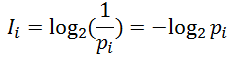
为了计算熵,我们需要计算所有类别所有可能值包含的信息期望值,通过下面的公式得到:
其中pi表示第i个类别在整个训练元组中出现的概率,可以用属于此类别元素的数量除以训练元组元素总数量作为估计。熵的实际意义表示是D中元组的类标号所需要的平均信息量
决策树和信息增益的理解:
https://blog.csdn.net/mn_kw/article/details/79913786
https://www.cnblogs.com/muzixi/p/6566803.html
ID3算法就是在每次需要分裂时,计算每个属性的增益率,然后选择增益率最大的属性进行分裂
code_lr_svm
#读取特征
import time
import pickle
from sklearn.feature_selection import SelectFromModel
from sklearn.linear_model import LogisticRegression
from sklearn.svm import LinearSVC
from sklearn.model_selection import train_test_split
from sklearn.metrics import confusion_matrix,f1_score

features_path = './feature/feature_file/data_w_tfidf.pkl'#tfidf特征的路径
fp = open(features_path, 'rb')
x_train, y_train, x_test = pickle.load(fp)
fp.close()
#将前面进行TF-IDF的数据中训练集 拆成 train_data, valid_data, 调最优模型参数,再进行测试
x_train1, x_valid,y_train1, y_valid = train_test_split(x_train, y_train, test_size=0.3, random_state=2019)
# 选取部分数据跑LR/SVM模型,判断结果。
print('模型训练结果')
svm=LinearSVC(C=5, dual=False)
log=LogisticRegression(class_weight='balanced')
for model in ((svm,log)):
    model.fit(x_train1,y_train1)
    predicted_value=model.predict(x_valid)
    score=model.score(x_valid,y_valid)
    matrix=confusion_matrix(y_valid,predicted_value)
    print(model)
    print('f值:',f1_score(y_valid,predicted_value,average='micro'))
    print('Score:',score)
#     print('matrix:',matrix)
模型训练结果
LinearSVC(C=5, class_weight=None, dual=False, fit_intercept=True,
     intercept_scaling=1, loss='squared_hinge', max_iter=1000,
     multi_class='ovr', penalty='l2', random_state=None, tol=0.0001,
     verbose=0)
f值: 0.7446666666666667
Score: 0.7446666666666667
LogisticRegression(C=1.0, class_weight='balanced', dual=False,
          fit_intercept=True, intercept_scaling=1, max_iter=100,
          multi_class='ovr', n_jobs=1, penalty='l2', random_state=None,
          solver='liblinear', tol=0.0001, verbose=0, warm_start=False)
f值: 0.704
Score: 0.704
# 特征选择
# sklearn在Feature selection模块中内置了一个SelectFromModel,该模型可以通过Model本身给出的指标对特征进行选择,
# 可参考https://blog.csdn.net/fontthrone/article/details/79064930
# eg:
# model = SelectFromModel(svm,prefit=True)
# X_new = model.transform(X)
# print(“X_new 共有 %s 个特征”%X_new.shape[1])
# 特征选取并不一定升:所有特征有效的情况下,去除的特征只能带来模型性能的下降,即使不是全部有效很多时候,低重要程度的特征也并不一定代表着一定会导致模型性能的下降,
# 因为某种度量方式并不代表着该特征的最终效果,很多时候我们的度量方式,往往只是一个参考而已.
# 跑随机森林模型
from sklearn.ensemble import RandomForestClassifier
# x_train1, x_valid,y_train1, y_valid = train_test_split(x_train, y_train, test_size=0.3, random_state=2019)
X_train, X_test, Y_train, Y_test = train_test_split(x_train, y_train, test_size=0.3, random_state=2019)
#初始化分类器
clf=RandomForestClassifier(n_estimators=500, criterion='entropy', max_depth=5, min_samples_split=2,
min_samples_leaf=1, max_features='auto', bootstrap=False, oob_score=False, n_jobs=1, random_state=0,
verbose=0)
X_train.shape
Y_train.shape
(3500, 190267)


(3500,)
###grid search找到最好的参数
from sklearn.pipeline import Pipeline
from sklearn.model_selection import GridSearchCV
from  sklearn.model_selection import StratifiedShuffleSplit


param_grid = dict( )
##创建分类pipeline
pipeline=Pipeline([ ('clf',clf) ])
grid_search = GridSearchCV(pipeline, param_grid=param_grid, verbose=3,scoring='accuracy',
cv=StratifiedShuffleSplit(n_splits=10,test_size=0.2, random_state=0)).fit(X_train, Y_train)
Fitting 10 folds for each of 1 candidates, totalling 10 fits
[CV]  ................................................................
[CV] ....................... , score=0.4328571428571429, total=  11.0s
[CV]  ................................................................


[Parallel(n_jobs=1)]: Done   1 out of   1 | elapsed:   15.2s remaining:    0.0s


[CV] ...................... , score=0.41285714285714287, total=  10.6s
[CV]  ................................................................


[Parallel(n_jobs=1)]: Done   2 out of   2 | elapsed:   30.1s remaining:    0.0s


[CV] ....................... , score=0.3985714285714286, total=  10.6s
[CV]  ................................................................
[CV] ....................... , score=0.4014285714285714, total=  13.2s
[CV]  ................................................................
[CV] ....................... , score=0.4342857142857143, total=  12.1s
[CV]  ................................................................
[CV] ...................... , score=0.42428571428571427, total=  13.5s
[CV]  ................................................................
[CV] ...................... , score=0.42714285714285716, total=  11.0s
[CV]  ................................................................
[CV] ..................................... , score=0.41, total=  12.3s
[CV]  ................................................................
[CV] ..................................... , score=0.42, total=  12.9s
[CV]  ................................................................
[CV] ...................... , score=0.42428571428571427, total=  12.9s


[Parallel(n_jobs=1)]: Done  10 out of  10 | elapsed:  2.8min finished
X_train.shape
Y_train.shape
(3500, 190267)


(3500,)
#####调参, 可用sklearn.pipeline
from sklearn.pipeline import Pipeline
from operator import itemgetter
import collections
from sklearn.metrics import classification_report
from sklearn.model_selection import cross_val_score

def report(grid_scores, n_top=3):
    top_scores = sorted(grid_scores, key=itemgetter(1), reverse=True)[:n_top]
    for i, score in enumerate(top_scores):
        print("Model with rank: {0}".format(i + 1))
        print("Mean validation score: {0:.3f} (std: {1:.3f})".format(
                score.mean_validation_score,
                np.std(score.cv_validation_scores)))
        print("Parameters: {0}".format(score.parameters))
        print("")
## 输出最优结果
from sklearn.model_selection import cross_val_score

print(("Best score: %0.3f" % grid_search.best_score_))
print((grid_search.best_estimator_))
#report(grid_search.best_score_)

print('-----grid search end------------')

print ('on all train set')

scores = cross_val_score(grid_search.best_estimator_, X_train, Y_train,cv=3,scoring='accuracy')
print("1111")
print(scores.mean(),scores)
print ('on test set')
scores = cross_val_score(grid_search.best_estimator_, X_test, Y_test,cv=3,scoring='accuracy')
print(scores.mean(),scores)
print((classification_report(Y_train, grid_search.best_estimator_.predict(X_train) )))
print('test data')
print((classification_report(Y_test, grid_search.best_estimator_.predict(X_test) )))
Best score: 0.419
Pipeline(memory=None,
     steps=[('clf', RandomForestClassifier(bootstrap=False, class_weight=None,
            criterion='entropy', max_depth=5, max_features='auto',
            max_leaf_nodes=None, min_impurity_decrease=0.0,
            min_impurity_split=None, min_samples_leaf=1,
            min_samples_split=2, min_weight_fraction_leaf=0.0,
            n_estimators=500, n_jobs=1, oob_score=False, random_state=0,
            verbose=0, warm_start=False))])
-----grid search end------------
on all train set
1111
0.4096658712329404 [0.41858483 0.41730934 0.39310345]
on test set
0.36470047260859656 [0.37080868 0.33867735 0.38461538]


D:\ProgramData\Anaconda3\lib\site-packages\sklearn\metrics\classification.py:1135: UndefinedMetricWarning: Precision and F-score are ill-defined and being set to 0.0 in labels with no predicted samples.
  'precision', 'predicted', average, warn_for)


             precision    recall  f1-score   support

          0       1.00      0.08      0.15       195
          1       1.00      0.11      0.20       100
          2       0.59      0.79      0.68       272
          3       1.00      0.22      0.36       139
          4       1.00      0.02      0.05        81
          5       0.94      0.71      0.81       239
          6       1.00      0.09      0.17       121
          7       0.44      0.85      0.58       245
          8       0.80      0.93      0.86       239
          9       1.00      0.08      0.15       150
         10       0.00      0.00      0.00       118
         11       1.00      0.03      0.05       177
         12       0.50      0.82      0.62       268
         13       0.64      0.81      0.71       232
         14       0.24      0.94      0.38       288
         15       0.00      0.00      0.00       110
         16       1.00      0.01      0.02       110
         17       0.84      0.77      0.80       222
         18       1.00      0.10      0.18       194

avg / total       0.71      0.51      0.44      3500

test data
             precision    recall  f1-score   support

          0       0.00      0.00      0.00        67
          1       0.00      0.00      0.00        39
          2       0.48      0.61      0.53       127
          3       1.00      0.08      0.14        52
          4       0.00      0.00      0.00        33
          5       0.88      0.63      0.73       110
          6       0.00      0.00      0.00        50
          7       0.32      0.76      0.45        94
          8       0.74      0.84      0.79       115
          9       1.00      0.01      0.03        69
         10       0.00      0.00      0.00        41
         11       0.00      0.00      0.00        83
         12       0.48      0.70      0.57       137
         13       0.56      0.71      0.62        96
         14       0.18      0.85      0.30       108
         15       0.00      0.00      0.00        49
         16       0.00      0.00      0.00        48
         17       0.70      0.59      0.64        91
         18       0.00      0.00      0.00        91

avg / total       0.40      0.42      0.35      1500
datawhale day05
【Task3.2】LightGBM模型(2天)
构建LightGBM的模型(包括:模型构建&调参&性能评估),学习理论并用Task2的特征实践
要求:理论+代码+截图F1评分的结果
LightGBM简介
LightGBM是一个梯度Boosting框架,使用基于决策树的学习算法。它可以说是分布式的,高效的,有以下优势:
1)更快的训练效率
2)低内存使用
3)更高的准确率
4)支持并行化学习
5)可以处理大规模数据
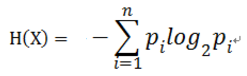
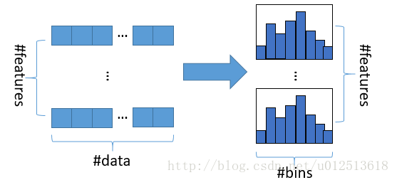
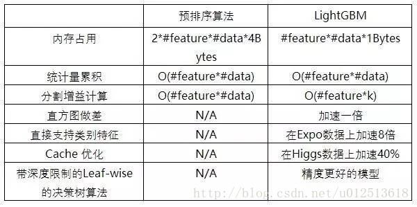
与常见的机器学习算法对比,速度是非常快的
XGboost的缺点
在讨论LightGBM时,不可避免的会提到XGboost,关于XGboost可以参考此博文
关于XGboost的不足之处主要有:
1)每轮迭代时,都需要遍历整个训练数据多次。如果把整个训练数据装进内存则会限制训练数据的大小;如果不装进内存,反复地读写训练数据又会消耗非常大的时间。
2)预排序方法的时间和空间的消耗都很大
LightGBM原理
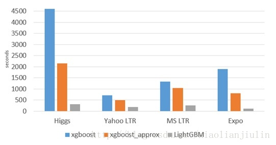
1)直方图算法
直方图算法的基本思想是先把连续的浮点特征值离散化成k个整数,同时构造一个宽度为k的直方图。在遍历数据的时候,根据离散化后的值作为索引在直方图中累积统计量,当遍历一次数据后,直方图累积了需要的统计量,然后根据直方图的离散值,遍历寻找最优的分割点。在XGBoost中需要遍历所有离散化的值,而在这里只要遍历k个直方图的值。
使用直方图算法有很多优点。首先,最明显就是内存消耗的降低,直方图算法不仅不需要额外存储预排序的结果,而且可以只保存特征离散化后的值。
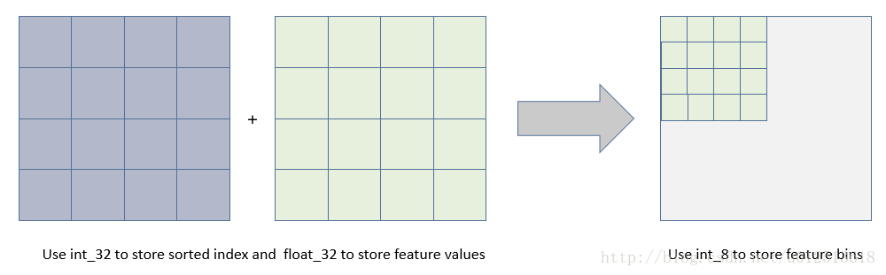
然后在计算上的代价也大幅降低,XGBoost预排序算法每遍历一个特征值就需要计算一次分裂的增益,而直方图算法只需要计算k次(k可以认为是常数),时间复杂度从O(#data * #feature) 优化到O(k* #features)。
当然,Histogram算法并不是完美的。由于特征被离散化后,找到的并不是很精确的分割点,所以会对结果产生影响。但在不同的数据集上的结果表明,离散化的分割点对最终的精度影响并不是很大,甚至有时候会更好一点。原因是决策树本来就是弱模型,分割点是不是精确并不是太重要;较粗的分割点也有正则化的效果,可以有效地防止过拟合;即使单棵树的训练误差比精确分割的算法稍大,但在梯度提升(Gradient Boosting)的框架下没有太大的影响。
2)LightGBM的直方图做差加速
一个容易观察到的现象:一个叶子的直方图可以由它的父亲节点的直方图与它兄弟的直方图做差得到。通常构造直方图,需要遍历该叶子上的所有数据,但直方图做差仅需遍历直方图的k个桶。利用这个方法,LightGBM可以在构造一个叶子的直方图后(父节点在上一轮就已经计算出来了),可以用非常微小的代价得到它兄弟叶子的直方图,在速度上可以提升一倍。

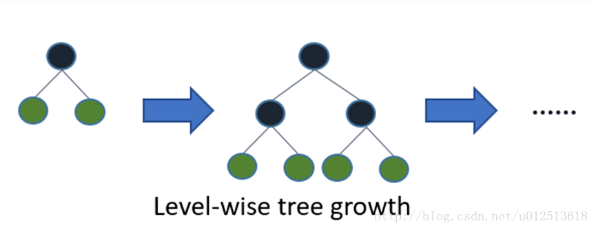
3)带深度限制的Leaf-wise的叶子生长策略
Level-wise过一次数据可以同时分裂同一层的叶子,容易进行多线程优化,也好控制模型复杂度,不容易过拟合。但实际上Level-wise是一种低效的算法,因为它不加区分的对待同一层的叶子,带来了很多没必要的开销,因为实际上很多叶子的分裂增益较低,没必要进行搜索和分裂。
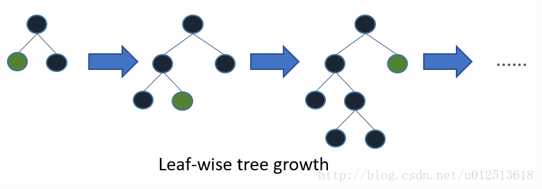
Leaf-wise则是一种更为高效的策略,每次从当前所有叶子中,找到分裂增益最大的一个叶子,然后分裂,如此循环。因此同Level-wise相比,在分裂次数相同的情况下,Leaf-wise可以降低更多的误差,得到更好的精度。Leaf-wise的缺点是可能会长出比较深的决策树,产生过拟合。因此LightGBM在Leaf-wise之上增加了一个最大深度的限制,在保证高效率的同时防止过拟合。
4)直接支持类别特征(即不需要做one-hot编码)
实际上大多数机器学习工具都无法直接支持类别特征,一般需要把类别特征,转化到多维的one-hot编码特征,降低了空间和时间的效率。而类别特征的使用是在实践中很常用的。基于这个考虑,LightGBM优化了对类别特征的支持,可以直接输入类别特征,不需要额外的one-hot编码展开。并在决策树算法上增加了类别特征的决策规则。在Expo数据集上的实验,相比0/1展开的方法,训练速度可以加速8倍,并且精度一致。
5)直接支持高效并行
LightGBM还具有支持高效并行的优点。LightGBM原生支持并行学习,目前支持特征并行和数据并行的两种。
1)特征并行的主要思想是在不同机器在不同的特征集合上分别寻找最优的分割点,然后在机器间同步最优的分割点。
2)数据并行则是让不同的机器先在本地构造直方图,然后进行全局的合并,最后在合并的直方图上面寻找最优分割点。
LightGBM针对这两种并行方法都做了优化,在特征并行算法中,通过在本地保存全部数据避免对数据切分结果的通信;在数据并行中使用分散规约 (Reduce scatter) 把直方图合并的任务分摊到不同的机器,降低通信和计算,并利用直方图做差,进一步减少了一半的通信量。


…
LightGBM参数调优
下面几张表为重要参数的含义和如何应用
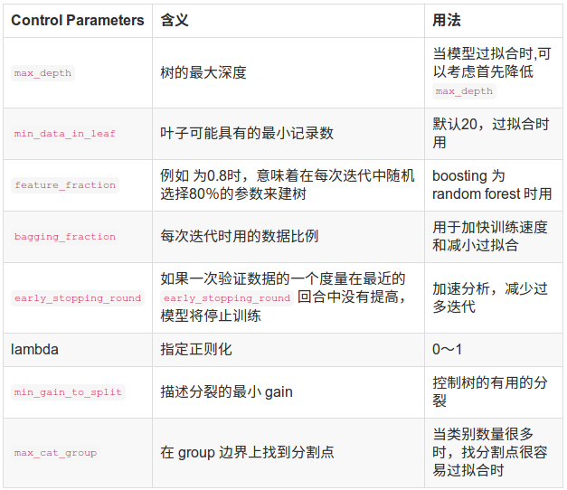
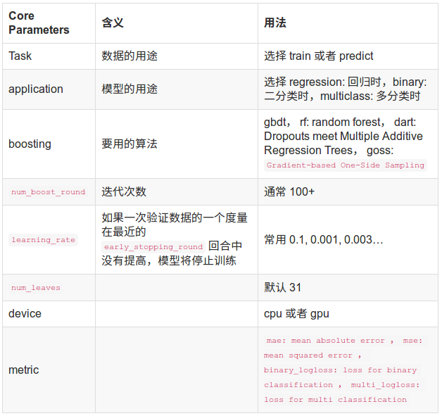
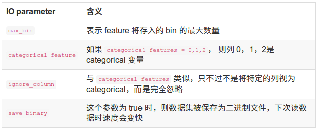
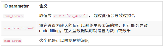
接下来是调参
下表对应了Faster Spread,better accuracy,over-fitting三种目的时,可以调整的参数
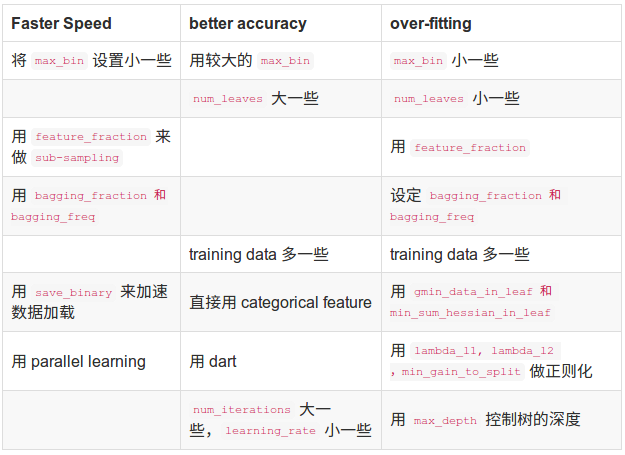
参考:https://www.cnblogs.com/jiangxinyang/p/9337094.html
code_LightGBM
#####跑LightGBM
import time
import pickle
import lightgbm as lgb
from sklearn.externals import joblib
from sklearn.model_selection import train_test_split, StratifiedKFold
from sklearn.metrics import f1_score,recall_score,accuracy_score,confusion_matrix
import numpy as np
import pandas as pd
t_start = time.time()
features_path = './feature/feature_file/data_w_tfidf.pkl'#tfidf特征的路径
fp = open(features_path, 'rb')
x_train, y_train, x_test = pickle.load(fp)
fp.close()
X_train, X_valid, y_train, y_valid = train_test_split(x_train, y_train, test_size=0.3,shuffle=True, random_state=2019)
#自定义验证集的评价函数
def f1_score_vali(preds, data_vali):
    labels = data_vali.get_label()
    print (labels.shape)
#     preds = np.argmax(preds.reshape(20, -1), axis=0)
    preds = np.argmax(preds.reshape(19, -1), axis=0)
    score_vali = f1_score(y_true=labels, y_pred=preds, average='macro')
    return 'f1_score', score_vali, True
#读取数据,并转换到lgb的标准数据格式
lgb_train = lgb.Dataset(X_train, y_train)
lgb_eval = lgb.Dataset(X_valid, y_valid, reference=lgb_train)
#nfold = 5
#kf = StratifiedKFold(nfold)
#训练lgb分类器
params = {
        'boosting': 'gbdt',
        'application': 'multiclass',
        'num_class': 19,
        'learning_rate': 0.1,
        'num_leaves': 31,
        'max_depth': -1,
        'lambda_l1': 0,
        'lambda_l2': 0.5,
        'bagging_fraction': 1.0,
        }
lgb_model = lgb.train(params, lgb_train, num_boost_round = 200, valid_sets = lgb_eval, feval =f1_score_vali,
                      early_stopping_rounds = None, verbose_eval=True)
(1500,)
[1]	valid_0's multi_logloss: 2.59063	valid_0's f1_score: 0.358601


D:\ProgramData\Anaconda3\lib\site-packages\sklearn\metrics\classification.py:1135: UndefinedMetricWarning: F-score is ill-defined and being set to 0.0 in labels with no predicted samples.
  'precision', 'predicted', average, warn_for)


(1500,)
[2]	valid_0's multi_logloss: 2.42449	valid_0's f1_score: 0.455623
(1500,)
[3]	valid_0's multi_logloss: 2.30233	valid_0's f1_score: 0.484192
(1500,)
[4]	valid_0's multi_logloss: 2.2055	valid_0's f1_score: 0.507549
(1500,)
[5]	valid_0's multi_logloss: 2.12282	valid_0's f1_score: 0.514249
(1500,)
[6]	valid_0's multi_logloss: 2.05372	valid_0's f1_score: 0.525165
(1500,)
[7]	valid_0's multi_logloss: 1.98988	valid_0's f1_score: 0.539878
(1500,)
[8]	valid_0's multi_logloss: 1.93636	valid_0's f1_score: 0.535049
(1500,)
[9]	valid_0's multi_logloss: 1.8873	valid_0's f1_score: 0.536848
(1500,)
[10]	valid_0's multi_logloss: 1.84304	valid_0's f1_score: 0.542822
(1500,)
[11]	valid_0's multi_logloss: 1.80461	valid_0's f1_score: 0.544681
(1500,)
[12]	valid_0's multi_logloss: 1.76446	valid_0's f1_score: 0.547263
(1500,)
[13]	valid_0's multi_logloss: 1.73078	valid_0's f1_score: 0.555018
(1500,)
[14]	valid_0's multi_logloss: 1.6997	valid_0's f1_score: 0.552516
(1500,)
[15]	valid_0's multi_logloss: 1.67258	valid_0's f1_score: 0.559633
(1500,)
[16]	valid_0's multi_logloss: 1.64422	valid_0's f1_score: 0.558745
(1500,)
[17]	valid_0's multi_logloss: 1.61952	valid_0's f1_score: 0.560212
(1500,)
[18]	valid_0's multi_logloss: 1.59664	valid_0's f1_score: 0.564883
(1500,)
[19]	valid_0's multi_logloss: 1.57363	valid_0's f1_score: 0.571394
(1500,)
[20]	valid_0's multi_logloss: 1.5545	valid_0's f1_score: 0.569059
(1500,)
[21]	valid_0's multi_logloss: 1.53565	valid_0's f1_score: 0.571338
(1500,)
[22]	valid_0's multi_logloss: 1.51683	valid_0's f1_score: 0.577117
(1500,)
[23]	valid_0's multi_logloss: 1.49951	valid_0's f1_score: 0.576341
(1500,)
[24]	valid_0's multi_logloss: 1.48304	valid_0's f1_score: 0.581325
(1500,)
[25]	valid_0's multi_logloss: 1.46871	valid_0's f1_score: 0.583088
(1500,)
[26]	valid_0's multi_logloss: 1.45543	valid_0's f1_score: 0.581542
(1500,)
[27]	valid_0's multi_logloss: 1.44104	valid_0's f1_score: 0.590096
(1500,)
[28]	valid_0's multi_logloss: 1.42792	valid_0's f1_score: 0.593722
(1500,)
[29]	valid_0's multi_logloss: 1.41534	valid_0's f1_score: 0.596916
(1500,)
[30]	valid_0's multi_logloss: 1.40501	valid_0's f1_score: 0.595933
(1500,)
[31]	valid_0's multi_logloss: 1.39541	valid_0's f1_score: 0.596998
(1500,)
[32]	valid_0's multi_logloss: 1.38384	valid_0's f1_score: 0.60193
(1500,)
[33]	valid_0's multi_logloss: 1.37403	valid_0's f1_score: 0.602808
(1500,)
[34]	valid_0's multi_logloss: 1.36561	valid_0's f1_score: 0.600789
(1500,)
[35]	valid_0's multi_logloss: 1.35692	valid_0's f1_score: 0.602871
(1500,)
[36]	valid_0's multi_logloss: 1.3477	valid_0's f1_score: 0.603776
(1500,)
[37]	valid_0's multi_logloss: 1.33975	valid_0's f1_score: 0.600854
(1500,)
[38]	valid_0's multi_logloss: 1.33184	valid_0's f1_score: 0.60274
(1500,)
[39]	valid_0's multi_logloss: 1.32426	valid_0's f1_score: 0.604953
(1500,)
[40]	valid_0's multi_logloss: 1.31794	valid_0's f1_score: 0.606162
(1500,)
[41]	valid_0's multi_logloss: 1.31084	valid_0's f1_score: 0.608378
(1500,)
[42]	valid_0's multi_logloss: 1.30302	valid_0's f1_score: 0.609082
(1500,)
[43]	valid_0's multi_logloss: 1.29701	valid_0's f1_score: 0.609802
(1500,)
[44]	valid_0's multi_logloss: 1.29103	valid_0's f1_score: 0.61324
(1500,)
[45]	valid_0's multi_logloss: 1.28423	valid_0's f1_score: 0.611178
(1500,)
[46]	valid_0's multi_logloss: 1.27831	valid_0's f1_score: 0.616824
(1500,)
[47]	valid_0's multi_logloss: 1.27417	valid_0's f1_score: 0.616864
(1500,)
[48]	valid_0's multi_logloss: 1.26778	valid_0's f1_score: 0.613787
(1500,)
[49]	valid_0's multi_logloss: 1.26316	valid_0's f1_score: 0.616183
(1500,)
[50]	valid_0's multi_logloss: 1.25853	valid_0's f1_score: 0.616038
(1500,)
[51]	valid_0's multi_logloss: 1.25564	valid_0's f1_score: 0.610348
(1500,)
[52]	valid_0's multi_logloss: 1.25087	valid_0's f1_score: 0.612741
(1500,)
[53]	valid_0's multi_logloss: 1.24665	valid_0's f1_score: 0.613516
(1500,)
[54]	valid_0's multi_logloss: 1.2433	valid_0's f1_score: 0.613313
(1500,)
[55]	valid_0's multi_logloss: 1.23971	valid_0's f1_score: 0.612886
(1500,)
[56]	valid_0's multi_logloss: 1.23546	valid_0's f1_score: 0.608856
(1500,)
[57]	valid_0's multi_logloss: 1.23247	valid_0's f1_score: 0.609235
(1500,)
[58]	valid_0's multi_logloss: 1.23006	valid_0's f1_score: 0.609003
(1500,)
[59]	valid_0's multi_logloss: 1.22679	valid_0's f1_score: 0.610566
(1500,)
[60]	valid_0's multi_logloss: 1.22524	valid_0's f1_score: 0.606199
(1500,)
[61]	valid_0's multi_logloss: 1.22288	valid_0's f1_score: 0.603776
(1500,)
[62]	valid_0's multi_logloss: 1.22003	valid_0's f1_score: 0.605379
(1500,)
[63]	valid_0's multi_logloss: 1.21726	valid_0's f1_score: 0.606571
(1500,)
[64]	valid_0's multi_logloss: 1.21455	valid_0's f1_score: 0.605871
(1500,)
[65]	valid_0's multi_logloss: 1.21277	valid_0's f1_score: 0.606017
(1500,)
[66]	valid_0's multi_logloss: 1.21102	valid_0's f1_score: 0.606701
(1500,)
[67]	valid_0's multi_logloss: 1.2101	valid_0's f1_score: 0.611597
(1500,)
[68]	valid_0's multi_logloss: 1.208	valid_0's f1_score: 0.611618
(1500,)
[69]	valid_0's multi_logloss: 1.20559	valid_0's f1_score: 0.61182
(1500,)
[70]	valid_0's multi_logloss: 1.20279	valid_0's f1_score: 0.610462
(1500,)
[71]	valid_0's multi_logloss: 1.20151	valid_0's f1_score: 0.612281
(1500,)
[72]	valid_0's multi_logloss: 1.19972	valid_0's f1_score: 0.611773
(1500,)
[73]	valid_0's multi_logloss: 1.19975	valid_0's f1_score: 0.614369
(1500,)
[74]	valid_0's multi_logloss: 1.19924	valid_0's f1_score: 0.614281
(1500,)
[75]	valid_0's multi_logloss: 1.19789	valid_0's f1_score: 0.61395
(1500,)
[76]	valid_0's multi_logloss: 1.19645	valid_0's f1_score: 0.613133
(1500,)
[77]	valid_0's multi_logloss: 1.19537	valid_0's f1_score: 0.612586
(1500,)
[78]	valid_0's multi_logloss: 1.19498	valid_0's f1_score: 0.611804
(1500,)
[79]	valid_0's multi_logloss: 1.19434	valid_0's f1_score: 0.612644
(1500,)
[80]	valid_0's multi_logloss: 1.19394	valid_0's f1_score: 0.616274
(1500,)
[81]	valid_0's multi_logloss: 1.19399	valid_0's f1_score: 0.615787
(1500,)
[82]	valid_0's multi_logloss: 1.19333	valid_0's f1_score: 0.615614
(1500,)
[83]	valid_0's multi_logloss: 1.19259	valid_0's f1_score: 0.618481
(1500,)
[84]	valid_0's multi_logloss: 1.19226	valid_0's f1_score: 0.619502
(1500,)
[85]	valid_0's multi_logloss: 1.1921	valid_0's f1_score: 0.620094
(1500,)
[86]	valid_0's multi_logloss: 1.19166	valid_0's f1_score: 0.620742
(1500,)
[87]	valid_0's multi_logloss: 1.1914	valid_0's f1_score: 0.619115
(1500,)
[88]	valid_0's multi_logloss: 1.19091	valid_0's f1_score: 0.619807
(1500,)
[89]	valid_0's multi_logloss: 1.19084	valid_0's f1_score: 0.620662
(1500,)
[90]	valid_0's multi_logloss: 1.19117	valid_0's f1_score: 0.619772
(1500,)
[91]	valid_0's multi_logloss: 1.19117	valid_0's f1_score: 0.618016
(1500,)
[92]	valid_0's multi_logloss: 1.19181	valid_0's f1_score: 0.620619
(1500,)
[93]	valid_0's multi_logloss: 1.19185	valid_0's f1_score: 0.619852
(1500,)
[94]	valid_0's multi_logloss: 1.19129	valid_0's f1_score: 0.62038
(1500,)
[95]	valid_0's multi_logloss: 1.19224	valid_0's f1_score: 0.621833
(1500,)
[96]	valid_0's multi_logloss: 1.19182	valid_0's f1_score: 0.624141
(1500,)
[97]	valid_0's multi_logloss: 1.19162	valid_0's f1_score: 0.623227
(1500,)
[98]	valid_0's multi_logloss: 1.19184	valid_0's f1_score: 0.6233
(1500,)
[99]	valid_0's multi_logloss: 1.19103	valid_0's f1_score: 0.624119
(1500,)
[100]	valid_0's multi_logloss: 1.19162	valid_0's f1_score: 0.627085
(1500,)
[101]	valid_0's multi_logloss: 1.19243	valid_0's f1_score: 0.624832
(1500,)
[102]	valid_0's multi_logloss: 1.19204	valid_0's f1_score: 0.628537
(1500,)
[103]	valid_0's multi_logloss: 1.19251	valid_0's f1_score: 0.627091
(1500,)
[104]	valid_0's multi_logloss: 1.19279	valid_0's f1_score: 0.625514
(1500,)
[105]	valid_0's multi_logloss: 1.19388	valid_0's f1_score: 0.622986
(1500,)
[106]	valid_0's multi_logloss: 1.19393	valid_0's f1_score: 0.623407
(1500,)
[107]	valid_0's multi_logloss: 1.19435	valid_0's f1_score: 0.623821
(1500,)
[108]	valid_0's multi_logloss: 1.19513	valid_0's f1_score: 0.627616
(1500,)
[109]	valid_0's multi_logloss: 1.19596	valid_0's f1_score: 0.627122
(1500,)
[110]	valid_0's multi_logloss: 1.19605	valid_0's f1_score: 0.625824
(1500,)
[111]	valid_0's multi_logloss: 1.1959	valid_0's f1_score: 0.627611
(1500,)
[112]	valid_0's multi_logloss: 1.19671	valid_0's f1_score: 0.629183
(1500,)
[113]	valid_0's multi_logloss: 1.19724	valid_0's f1_score: 0.628136
(1500,)
[114]	valid_0's multi_logloss: 1.19804	valid_0's f1_score: 0.625342
(1500,)
[115]	valid_0's multi_logloss: 1.1979	valid_0's f1_score: 0.6256
(1500,)
[116]	valid_0's multi_logloss: 1.19832	valid_0's f1_score: 0.626885
(1500,)
[117]	valid_0's multi_logloss: 1.19904	valid_0's f1_score: 0.626052
(1500,)
[118]	valid_0's multi_logloss: 1.20013	valid_0's f1_score: 0.626607
(1500,)
[119]	valid_0's multi_logloss: 1.20077	valid_0's f1_score: 0.627361
(1500,)
[120]	valid_0's multi_logloss: 1.20095	valid_0's f1_score: 0.626664
(1500,)
[121]	valid_0's multi_logloss: 1.20177	valid_0's f1_score: 0.625271
(1500,)
[122]	valid_0's multi_logloss: 1.20159	valid_0's f1_score: 0.625527
(1500,)
[123]	valid_0's multi_logloss: 1.20212	valid_0's f1_score: 0.626395
(1500,)
[124]	valid_0's multi_logloss: 1.20191	valid_0's f1_score: 0.62578
(1500,)
[125]	valid_0's multi_logloss: 1.20262	valid_0's f1_score: 0.626537
(1500,)
[126]	valid_0's multi_logloss: 1.20432	valid_0's f1_score: 0.625898
(1500,)
[127]	valid_0's multi_logloss: 1.20487	valid_0's f1_score: 0.62681
(1500,)
[128]	valid_0's multi_logloss: 1.20475	valid_0's f1_score: 0.626338
(1500,)
[129]	valid_0's multi_logloss: 1.20502	valid_0's f1_score: 0.625294
(1500,)
[130]	valid_0's multi_logloss: 1.20584	valid_0's f1_score: 0.624615
(1500,)
[131]	valid_0's multi_logloss: 1.20608	valid_0's f1_score: 0.624344
(1500,)
[132]	valid_0's multi_logloss: 1.20651	valid_0's f1_score: 0.621925
(1500,)
[133]	valid_0's multi_logloss: 1.20662	valid_0's f1_score: 0.622379
(1500,)
[134]	valid_0's multi_logloss: 1.20705	valid_0's f1_score: 0.622479
(1500,)
[135]	valid_0's multi_logloss: 1.20754	valid_0's f1_score: 0.622281
(1500,)
[136]	valid_0's multi_logloss: 1.20747	valid_0's f1_score: 0.624521
(1500,)
[137]	valid_0's multi_logloss: 1.20774	valid_0's f1_score: 0.624888
(1500,)
[138]	valid_0's multi_logloss: 1.2083	valid_0's f1_score: 0.625145
(1500,)
[139]	valid_0's multi_logloss: 1.20883	valid_0's f1_score: 0.625151
(1500,)
[140]	valid_0's multi_logloss: 1.20961	valid_0's f1_score: 0.624245
(1500,)
[141]	valid_0's multi_logloss: 1.21023	valid_0's f1_score: 0.624475
(1500,)
[142]	valid_0's multi_logloss: 1.21031	valid_0's f1_score: 0.624422
(1500,)
[143]	valid_0's multi_logloss: 1.21056	valid_0's f1_score: 0.623716
(1500,)
[144]	valid_0's multi_logloss: 1.21095	valid_0's f1_score: 0.62458
(1500,)
[145]	valid_0's multi_logloss: 1.21103	valid_0's f1_score: 0.625663
(1500,)
[146]	valid_0's multi_logloss: 1.21155	valid_0's f1_score: 0.625048
(1500,)
[147]	valid_0's multi_logloss: 1.2121	valid_0's f1_score: 0.6265
(1500,)
[148]	valid_0's multi_logloss: 1.2124	valid_0's f1_score: 0.626648
(1500,)
[149]	valid_0's multi_logloss: 1.21265	valid_0's f1_score: 0.624995
(1500,)
[150]	valid_0's multi_logloss: 1.21391	valid_0's f1_score: 0.625321
(1500,)
[151]	valid_0's multi_logloss: 1.21406	valid_0's f1_score: 0.625322
(1500,)
[152]	valid_0's multi_logloss: 1.21507	valid_0's f1_score: 0.624886
(1500,)
[153]	valid_0's multi_logloss: 1.21539	valid_0's f1_score: 0.623123
(1500,)
[154]	valid_0's multi_logloss: 1.21606	valid_0's f1_score: 0.624093
(1500,)
[155]	valid_0's multi_logloss: 1.21662	valid_0's f1_score: 0.624837
(1500,)
[156]	valid_0's multi_logloss: 1.21691	valid_0's f1_score: 0.624172
(1500,)
[157]	valid_0's multi_logloss: 1.21717	valid_0's f1_score: 0.623783
(1500,)
[158]	valid_0's multi_logloss: 1.21767	valid_0's f1_score: 0.62393
(1500,)
[159]	valid_0's multi_logloss: 1.21794	valid_0's f1_score: 0.623298
(1500,)
[160]	valid_0's multi_logloss: 1.21846	valid_0's f1_score: 0.623501
(1500,)
[161]	valid_0's multi_logloss: 1.21908	valid_0's f1_score: 0.622942
(1500,)
[162]	valid_0's multi_logloss: 1.21976	valid_0's f1_score: 0.621572
(1500,)
[163]	valid_0's multi_logloss: 1.22012	valid_0's f1_score: 0.621348
(1500,)
[164]	valid_0's multi_logloss: 1.22091	valid_0's f1_score: 0.622189
(1500,)
[165]	valid_0's multi_logloss: 1.22158	valid_0's f1_score: 0.622288
(1500,)
[166]	valid_0's multi_logloss: 1.22182	valid_0's f1_score: 0.623892
(1500,)
[167]	valid_0's multi_logloss: 1.22239	valid_0's f1_score: 0.623286
(1500,)
[168]	valid_0's multi_logloss: 1.22292	valid_0's f1_score: 0.623286
(1500,)
[169]	valid_0's multi_logloss: 1.22322	valid_0's f1_score: 0.624191
(1500,)
[170]	valid_0's multi_logloss: 1.22336	valid_0's f1_score: 0.623293
(1500,)
[171]	valid_0's multi_logloss: 1.22399	valid_0's f1_score: 0.622667
(1500,)
[172]	valid_0's multi_logloss: 1.22467	valid_0's f1_score: 0.622072
(1500,)
[173]	valid_0's multi_logloss: 1.22495	valid_0's f1_score: 0.622611
(1500,)
[174]	valid_0's multi_logloss: 1.22554	valid_0's f1_score: 0.622941
(1500,)
[175]	valid_0's multi_logloss: 1.22626	valid_0's f1_score: 0.622795
(1500,)
[176]	valid_0's multi_logloss: 1.22677	valid_0's f1_score: 0.622606
(1500,)
[177]	valid_0's multi_logloss: 1.2272	valid_0's f1_score: 0.621671
(1500,)
[178]	valid_0's multi_logloss: 1.22778	valid_0's f1_score: 0.622993
(1500,)
[179]	valid_0's multi_logloss: 1.22761	valid_0's f1_score: 0.622874
(1500,)
[180]	valid_0's multi_logloss: 1.22801	valid_0's f1_score: 0.621993
(1500,)
[181]	valid_0's multi_logloss: 1.22863	valid_0's f1_score: 0.621861
(1500,)
[182]	valid_0's multi_logloss: 1.22925	valid_0's f1_score: 0.622009
(1500,)
[183]	valid_0's multi_logloss: 1.2293	valid_0's f1_score: 0.622621
(1500,)
[184]	valid_0's multi_logloss: 1.2301	valid_0's f1_score: 0.622428
(1500,)
[185]	valid_0's multi_logloss: 1.23091	valid_0's f1_score: 0.622013
(1500,)
[186]	valid_0's multi_logloss: 1.23106	valid_0's f1_score: 0.621917
(1500,)
[187]	valid_0's multi_logloss: 1.23177	valid_0's f1_score: 0.62272
(1500,)
[188]	valid_0's multi_logloss: 1.23202	valid_0's f1_score: 0.622338
(1500,)
[189]	valid_0's multi_logloss: 1.23254	valid_0's f1_score: 0.623296
(1500,)
[190]	valid_0's multi_logloss: 1.23324	valid_0's f1_score: 0.623302
(1500,)
[191]	valid_0's multi_logloss: 1.23381	valid_0's f1_score: 0.623061
(1500,)
[192]	valid_0's multi_logloss: 1.23424	valid_0's f1_score: 0.62214
(1500,)
[193]	valid_0's multi_logloss: 1.23467	valid_0's f1_score: 0.622059
(1500,)
[194]	valid_0's multi_logloss: 1.23487	valid_0's f1_score: 0.622009
(1500,)
[195]	valid_0's multi_logloss: 1.23489	valid_0's f1_score: 0.623264
(1500,)
[196]	valid_0's multi_logloss: 1.23608	valid_0's f1_score: 0.622632
(1500,)
[197]	valid_0's multi_logloss: 1.23656	valid_0's f1_score: 0.622612
(1500,)
[198]	valid_0's multi_logloss: 1.237	valid_0's f1_score: 0.622503
(1500,)
[199]	valid_0's multi_logloss: 1.23764	valid_0's f1_score: 0.622612
(1500,)
[200]	valid_0's multi_logloss: 1.23797	valid_0's f1_score: 0.623156
# 保存模型
joblib.dump(lgb_model, "./lgb_w_tfidf.m")
['./lgb_w_tfidf.m']
##对测试集进行预测;将预测结果转换为官方标准格式;并将结果保存至本地
y_test = np.argmax(lgb_model.predict(x_test), axis=1) + 1
df_result = pd.DataFrame(data={'id':range(5000), 'class': y_test.tolist()})
result_path = './results/' + 'lgb' + '.csv'
print (result_path)
df_result.to_csv(result_path, index=False)

t_end = time.time()
print("训练结束,耗时:{}min".format((t_end - t_start) / 60))
./results/lgb.csv
训练结束,耗时:39.662170096238455min
datawhale_day06
数据竞赛 最终任务
【Task4 模型优化】:(2天)
1)进一步通过网格搜索法对3个模型进行调优(用5000条数据,调参时采用五折交叉验证的方式),并进行模型评估,展示代码的运行结果。(可以尝试使用其他模型)
2)模型融合,模型融合方式任意,并结合之前的任务给出你的最优结果。
例如Stacking融合,用你目前评分最高的模型作为基准模型,和其他模型进行stacking融合,得到最终模型及评分结果。
结果展示如下表:
| 模型 | 最优参数 | F1评分 | 训练耗时 |
|---|---|---|---|
| LR | Best parameters:{‘C’: 100} | 0.74 | 3.092217266559601min |
| SVM | Best parameters:{‘gamma’: 0.1, ‘C’: 100} | 0.73 | 26.319817582766216min |
| LightGBM | Best parameters:{‘gamma’: 0.001, ‘C’: 0.001} | 0.65 | 28.898845402399697min |
| 其他模型(XGBOST) | Best parameters:{‘gamma’: 0.01, ‘C’: 0.01} | 0.64 | 43.95693199634552min |
| 最优结果 | Best parameters:{‘gamma’: 0.01, ‘C’: 100} | 0.75 | 49.3455256931996min |
K折交叉验证&网格搜索法
K折交叉验证(k-fold cross validation),将初始采样(样本集X,Y)分割成K份,一份被保留作为验证模型的数据(test set),其他K-1份用来训练(train set)。交叉验证重复K次,每份验证一次,平均K次的结果或者使用其它结合方式,最终得到一个单一估测。
https://blog.csdn.net/tianguiyuyu/article/details/80697223
https://blog.csdn.net/zhaohaibo_/article/details/84619396
Grid Search:一种调参手段;穷举搜索:在所有候选的参数选择中,通过循环遍历,尝试每一种可能性,表现最好的参数就是最终的结果。其原理就像是在数组里找最大值。(为什么叫网格搜索?以有两个参数的模型为例,参数a有3种可能,参数b有4种可能,把所有可能性列出来,可以表示成一个3*4的表格,其中每个cell就是一个网格,循环过程就像是在每个网格里遍历、搜索,所以叫grid search)
https://www.cnblogs.com/ysugyl/p/8711205.html
https://www.cnblogs.com/nwpuxuezha/p/6618205.html
GridSearchCV & cross_val_score 思考
GridSearchCV(网格搜索)用简答的话来说就是你手动的给出一个模型中你想要改动的所用的参数,程序自动的帮你使用穷举法来将所用的参数都运行一遍。
cross_val_score 一般用于获取每折的交叉验证的得分,然后根据这个得分为模型选择合适的超参数,通常需要编写循环手动完成交叉验证过程;
GridSearchCV 除了自行完成叉验证外,还返回了最优的超参数及对应的最优模型
https://blog.csdn.net/weixin_40363627/article/details/85015683
code_模型调参
参考:https://blog.csdn.net/weixin_40363627/article/details/85015683
# 单行中间变量完全显示
from IPython.core.interactiveshell import InteractiveShell
InteractiveShell.ast_node_interactivity = "all"
#读取特征
import time
import pickle
from sklearn.feature_selection import SelectFromModel
from sklearn.linear_model import LogisticRegression
from sklearn.svm import LinearSVC
from sklearn.svm import SVC
from sklearn.model_selection import train_test_split
from sklearn.metrics import confusion_matrix,f1_score
from sklearn.model_selection import cross_val_score
import lightgbm as lgb
import xgboost as xgb


features_path = './feature/feature_file/data_w_tfidf.pkl'#tfidf特征的路径
fp = open(features_path, 'rb')
x_train, y_train, x_test = pickle.load(fp)
fp.close()
X_train, X_test, Y_train, Y_test = train_test_split(x_train, y_train, test_size=0.3, random_state=2019)
X_train.shape
y_train.shape
(3500, 190267)


(5000,)
# LR
t_start = time.time()
best_score = 0.0
# for gamma in [0.001,0.01,0.1,1,10,100]:
for C in [0.001,0.01,0.1,1,10,100]:
    log_model = LogisticRegression(C=C,random_state =2019)
    scores = cross_val_score(log_model,X_train,Y_train,cv=5) #5折交叉验证
    score = scores.mean() #取平均数
    if score > best_score:
        best_score = score
        best_parameters = {"C":C}
log_model = LogisticRegression(**best_parameters)
log_model.fit(X_train,Y_train)
test_score = log_model.score(X_test,Y_test)
print("Best score on validation set:{:.2f}".format(best_score))
print("Best parameters:{}".format(best_parameters))
print("Score on testing set:{:.2f}".format(test_score))
t_end = time.time()
print("训练结束,耗时:{}min".format((t_end - t_start) / 60))
LogisticRegression(C=100, class_weight=None, dual=False, fit_intercept=True,
          intercept_scaling=1, max_iter=100, multi_class='ovr', n_jobs=1,
          penalty='l2', random_state=None, solver='liblinear', tol=0.0001,
          verbose=0, warm_start=False)


Best score on validation set:0.70
Best parameters:{'C': 100}
Score on testing set:0.74
训练结束,耗时:3.092217266559601min
# svm
t_start = time.time()
best_score = 0.0
for gamma in [0.001,0.1]:
    for C in [10,100]:
# for gamma in [0.001,0.01,0.1,1,10,100]:
#     for C in [0.001,0.01,0.1,1,10,100]:
        svm = SVC(gamma=gamma,C=C,random_state =2019)
        scores = cross_val_score(svm,X_train,Y_train,cv=5) #5折交叉验证
        score = scores.mean() #取平均数
        if score > best_score:
            best_score = score
            best_parameters = {"gamma":gamma,"C":C}
svm = SVC(**best_parameters)
svm.fit(X_train,Y_train)
test_score = svm.score(X_test,Y_test)
print("Best score on validation set:{:.2f}".format(best_score))
print("Best parameters:{}".format(best_parameters))
print("Score on testing set:{:.2f}".format(test_score))
t_end = time.time()
print("训练结束,耗时:{}min".format((t_end - t_start) / 60))
SVC(C=100, cache_size=200, class_weight=None, coef0=0.0,
  decision_function_shape='ovr', degree=3, gamma=0.1, kernel='rbf',
  max_iter=-1, probability=False, random_state=None, shrinking=True,
  tol=0.001, verbose=False)


Best score on validation set:0.68
Best parameters:{'gamma': 0.1, 'C': 100}
Score on testing set:0.73
训练结束,耗时:26.319817582766216min
# lightGBM
t_start = time.time()
best_score = 0.0
# lgb_model = LGBMClassifier()

for gamma in [0.001,0.01]:
    for C in [0.001,0.01,]:
# for gamma in [0.001,0.01,0.1,1,10,100]:
#     for C in [0.001,0.01,0.1,1,10,100]:
        lgb_model = lgb.LGBMClassifier(gamma=gamma,C=C,random_state =2019)
        scores = cross_val_score(svm,X_train,Y_train,cv=5) #5折交叉验证
        score = scores.mean() #取平均数
        if score > best_score:
            best_score = score
            best_parameters = {"gamma":gamma,"C":C}
lgb_model = lgb.LGBMClassifier(**best_parameters)
lgb_model.fit(X_train,Y_train)
test_score = lgb_model.score(X_test,Y_test)
print("Best score on validation set:{:.2f}".format(best_score))
print("Best parameters:{}".format(best_parameters))
print("Score on testing set:{:.2f}".format(test_score))
t_end = time.time()
print("训练结束,耗时:{}min".format((t_end - t_start) / 60))
LGBMClassifier(C=0.001, boosting_type='gbdt', class_weight=None,
        colsample_bytree=1.0, gamma=0.001, importance_type='split',
        learning_rate=0.1, max_depth=-1, min_child_samples=20,
        min_child_weight=0.001, min_split_gain=0.0, n_estimators=100,
        n_jobs=-1, num_leaves=31, objective=None, random_state=None,
        reg_alpha=0.0, reg_lambda=0.0, silent=True, subsample=1.0,
        subsample_for_bin=200000, subsample_freq=0)


Best score on validation set:0.68
Best parameters:{'gamma': 0.001, 'C': 0.001}
Score on testing set:0.65
训练结束,耗时:28.898845402399697min


D:\ProgramData\Anaconda3\lib\site-packages\sklearn\preprocessing\label.py:151: DeprecationWarning: The truth value of an empty array is ambiguous. Returning False, but in future this will result in an error. Use `array.size > 0` to check that an array is not empty.
  if diff:
# XGBoost
t_start = time.time()
best_score = 0.0
# xgb_model = XGBClassifier()

for gamma in [0.01,0.1,]:
    for C in [0.01,0.1,]:

# for gamma in [0.001,0.01,0.1,1,10,100]:
#     for C in [0.001,0.01,0.1,1,10,100]:
        xgb_model = xgb.XGBClassifier(gamma=gamma,C=C,random_state =2018)
        scores = cross_val_score(svm,X_train,Y_train,cv=5) #5折交叉验证
        score = scores.mean() #取平均数
        if score > best_score:
            best_score = score
            best_parameters = {"gamma":gamma,"C":C}
xgb_model = xgb.XGBClassifier(**best_parameters)
xgb_model.fit(X_train,Y_train)
test_score = xgb_model.score(X_test,Y_test)
print("Best score on validation set:{:.2f}".format(best_score))
print("Best parameters:{}".format(best_parameters))
print("Score on testing set:{:.2f}".format(test_score))
t_end = time.time()
print("训练结束,耗时:{}min".format((t_end - t_start) / 60))
XGBClassifier(C=0.01, base_score=0.5, booster='gbtree', colsample_bylevel=1,
       colsample_bytree=1, gamma=0.01, learning_rate=0.1, max_delta_step=0,
       max_depth=3, min_child_weight=1, missing=None, n_estimators=100,
       n_jobs=1, nthread=None, objective='multi:softprob', random_state=0,
       reg_alpha=0, reg_lambda=1, scale_pos_weight=1, seed=None,
       silent=True, subsample=1)


Best score on validation set:0.68
Best parameters:{'gamma': 0.01, 'C': 0.01}
Score on testing set:0.64
训练结束,耗时:43.95693199634552min


D:\ProgramData\Anaconda3\lib\site-packages\sklearn\preprocessing\label.py:151: DeprecationWarning: The truth value of an empty array is ambiguous. Returning False, but in future this will result in an error. Use `array.size > 0` to check that an array is not empty.
  if diff:
code_模型融合
任务:
用你目前评分
最高的模型作为基准模型,和其他模型进行stacking融合,得到最终模型及评分果。
https://blog.csdn.net/weixin_40363627/article/details/86175919
CrossValidation 交叉验证和Stacking的深入理解
https://blog.csdn.net/herr_kun/article/details/84852280
# 单行中间变量完全显示
from IPython.core.interactiveshell import InteractiveShell
InteractiveShell.ast_node_interactivity = "all"
#读取特征

import time
import pandas as pd
import numpy as np
import sys
import pickle
from sklearn.model_selection import train_test_split
from sklearn.preprocessing import StandardScaler

from sklearn.linear_model import LogisticRegression
from sklearn.svm import SVC
from sklearn.tree import DecisionTreeClassifier
from sklearn.ensemble import RandomForestClassifier
from sklearn.ensemble import GradientBoostingClassifier
import xgboost as xgb
from xgboost import XGBClassifier
import lightgbm as lgb
from lightgbm import LGBMClassifier

from sklearn import metrics
import matplotlib.pyplot as plt

from sklearn.model_selection import KFold
from sklearn.model_selection import GridSearchCV
from sklearn.model_selection import cross_val_score
from sklearn.metrics import make_scorer
from sklearn.model_selection import cross_validate
from mlxtend.classifier import StackingClassifier


features_path = './feature/feature_file/data_w_tfidf.pkl'#tfidf特征的路径
fp = open(features_path, 'rb')
x_train, y_train, x_test = pickle.load(fp)
fp.close()
X_train, X_test, Y_train, Y_test = train_test_split(x_train, y_train, test_size=0.3, random_state=2019)
lr = LogisticRegression(random_state=2019,C=0.1)
lgb = LGBMClassifier(boosting_type='GBDT',random_state=2019,silent=0)
gbdt = GradientBoostingClassifier(random_state=2019,max_depth=3,n_estimators=50)
xgbc = XGBClassifier(random_state=2019,max_depth=3,eta=0.1,subsample=0.6)
rf = RandomForestClassifier(n_estimators=500,oob_score=True, random_state=2019)
svm = SVC(random_state=2019,tol=0.01)
sclf = StackingClassifier(classifiers=[lr, gbdt, xgbc,rf,svm], meta_classifier=lgb)

# sclf1 = StackingClassifier(classifiers=[gbdt, xgbc,svm], meta_classifier=lgb)
# sclf2 = StackingClassifier(classifiers=[gbdt, xgbc,svm], meta_classifier=lr)
# sclf3 = StackingClassifier(classifiers=[svm], meta_classifier=lr)
def get_scores(model, X_train, X_test, Y_train, Y_test):
    model.fit(X_train, Y_train)
    y_train_predict = model.predict(X_train)
    y_test_predict = model.predict(X_test)
    if hasattr(model, "decision_function"):
        y_train_proba = model.decision_function(X_train)
        y_test_proba = model.decision_function(X_test)
    else:
        y_train_proba = (model.predict_proba(X_train))[:, 1]
        y_test_proba = (model.predict_proba(X_test))[:, 1]
    # accuracy
    train_accuracy = metrics.accuracy_score(Y_train, y_train_predict)
    test_accuracy = metrics.accuracy_score(Y_test, y_test_predict)

    # recision
    train_precision = metrics.precision_score(Y_train, y_train_predict, average="micro")
    test_precision = metrics.precision_score(Y_test, y_test_predict, average="micro")

    # recall
    train_recall = metrics.recall_score(Y_train, y_train_predict, average="micro")
    test_recall = metrics.recall_score(Y_test, y_test_predict, average="micro")

    # f1-score
    train_f1 = metrics.f1_score(Y_train, y_train_predict, average="micro")
    test_f1 = metrics.f1_score(Y_test, y_test_predict, average="micro")

#     # auc
#     train_auc = metrics.roc_auc_score(Y_train, y_train_proba)
#     test_auc = metrics.roc_auc_score(Y_test, y_test_proba)
#     # roc 曲线
#     train_fprs,train_tprs,train_thresholds = metrics.roc_curve(Y_train, y_train_proba)
#     test_fprs,test_tprs,test_thresholds = metrics.roc_curve(Y_test, y_test_proba)
#     plt.plot(train_fprs, train_tprs)
#     plt.plot(test_fprs, test_tprs)
#     plt.plot([0,1], [0,1],"--")
#     plt.title("ROC curve")
#     plt.xlabel("FPR")
#     plt.ylabel("TPR")
#     plt.legend(labels=["Train AUC:"+str(round(train_auc, 5)),"Test AUC:"+str(round(test_auc,5))], loc="lower right")
#     plt.show()
    #输出各种得分
    print("训练集准确率:", train_accuracy)
    print("测试集准确率:", test_accuracy)
    print("==================================")
    print("训练集精准率:", train_precision)
    print("测试集精准率:", test_precision)
    print("==================================")
    print("训练集召回率:", train_recall)
    print("测试集召回率:", test_recall)
    print("==================================")
    print("训练集F1-score:", train_f1)
    print("测试集F1-score:", test_f1)
    print("==================================")
#     print("训练集AUC:", train_auc)
#     print("测试集AUC:", test_auc)
t_start = time.time()

get_scores(sclf, X_train, X_test, Y_train, Y_test)
t_end = time.time()
print("训练结束,耗时:{}min".format((t_end - t_start) / 60))
D:\ProgramData\Anaconda3\lib\site-packages\sklearn\preprocessing\label.py:151: DeprecationWarning: The truth value of an empty array is ambiguous. Returning False, but in future this will result in an error. Use `array.size > 0` to check that an array is not empty.
  if diff:
D:\ProgramData\Anaconda3\lib\site-packages\sklearn\preprocessing\label.py:151: DeprecationWarning: The truth value of an empty array is ambiguous. Returning False, but in future this will result in an error. Use `array.size > 0` to check that an array is not empty.
  if diff:
D:\ProgramData\Anaconda3\lib\site-packages\sklearn\preprocessing\label.py:151: DeprecationWarning: The truth value of an empty array is ambiguous. Returning False, but in future this will result in an error. Use `array.size > 0` to check that an array is not empty.
  if diff:
D:\ProgramData\Anaconda3\lib\site-packages\sklearn\preprocessing\label.py:151: DeprecationWarning: The truth value of an empty array is ambiguous. Returning False, but in future this will result in an error. Use `array.size > 0` to check that an array is not empty.
  if diff:
D:\ProgramData\Anaconda3\lib\site-packages\sklearn\preprocessing\label.py:151: DeprecationWarning: The truth value of an empty array is ambiguous. Returning False, but in future this will result in an error. Use `array.size > 0` to check that an array is not empty.
  if diff:
D:\ProgramData\Anaconda3\lib\site-packages\sklearn\preprocessing\label.py:151: DeprecationWarning: The truth value of an empty array is ambiguous. Returning False, but in future this will result in an error. Use `array.size > 0` to check that an array is not empty.
  if diff:
D:\ProgramData\Anaconda3\lib\site-packages\sklearn\preprocessing\label.py:151: DeprecationWarning: The truth value of an empty array is ambiguous. Returning False, but in future this will result in an error. Use `array.size > 0` to check that an array is not empty.
  if diff:


训练集准确率: 1.0
测试集准确率: 0.6073333333333333
==================================
训练集精准率: 1.0
测试集精准率: 0.6073333333333333
==================================
训练集召回率: 1.0
测试集召回率: 0.6073333333333333
==================================
训练集F1-score: 1.0
测试集F1-score: 0.6073333333333333
==================================
训练结束,耗时:45.054417494932814min
sclf1 = StackingClassifier(classifiers=[gbdt, xgbc,svm], meta_classifier=lgb)
sclf2 = StackingClassifier(classifiers=[gbdt, xgbc,svm], meta_classifier=lr)
sclf3 = StackingClassifier(classifiers=[svm], meta_classifier=lr)
t_start = time.time()

get_scores(sclf1, X_train, X_test, Y_train, Y_test)
t_end = time.time()
print("训练结束,耗时:{}min".format((t_end - t_start) / 60))
D:\ProgramData\Anaconda3\lib\site-packages\sklearn\preprocessing\label.py:151: DeprecationWarning: The truth value of an empty array is ambiguous. Returning False, but in future this will result in an error. Use `array.size > 0` to check that an array is not empty.
  if diff:
D:\ProgramData\Anaconda3\lib\site-packages\sklearn\preprocessing\label.py:151: DeprecationWarning: The truth value of an empty array is ambiguous. Returning False, but in future this will result in an error. Use `array.size > 0` to check that an array is not empty.
  if diff:
D:\ProgramData\Anaconda3\lib\site-packages\sklearn\preprocessing\label.py:151: DeprecationWarning: The truth value of an empty array is ambiguous. Returning False, but in future this will result in an error. Use `array.size > 0` to check that an array is not empty.
  if diff:
D:\ProgramData\Anaconda3\lib\site-packages\sklearn\preprocessing\label.py:151: DeprecationWarning: The truth value of an empty array is ambiguous. Returning False, but in future this will result in an error. Use `array.size > 0` to check that an array is not empty.
  if diff:
D:\ProgramData\Anaconda3\lib\site-packages\sklearn\preprocessing\label.py:151: DeprecationWarning: The truth value of an empty array is ambiguous. Returning False, but in future this will result in an error. Use `array.size > 0` to check that an array is not empty.
  if diff:
D:\ProgramData\Anaconda3\lib\site-packages\sklearn\preprocessing\label.py:151: DeprecationWarning: The truth value of an empty array is ambiguous. Returning False, but in future this will result in an error. Use `array.size > 0` to check that an array is not empty.
  if diff:
D:\ProgramData\Anaconda3\lib\site-packages\sklearn\preprocessing\label.py:151: DeprecationWarning: The truth value of an empty array is ambiguous. Returning False, but in future this will result in an error. Use `array.size > 0` to check that an array is not empty.
  if diff:


训练集准确率: 0.9937142857142857
测试集准确率: 0.6106666666666667
==================================
训练集精准率: 0.9937142857142857
测试集精准率: 0.6106666666666667
==================================
训练集召回率: 0.9937142857142857
测试集召回率: 0.6106666666666667
==================================
训练集F1-score: 0.9937142857142857
测试集F1-score: 0.6106666666666667
==================================
训练结束,耗时:46.9501273393631min
t_start = time.time()

get_scores(sclf2, X_train, X_test, Y_train, Y_test)
t_end = time.time()
print("训练结束,耗时:{}min".format((t_end - t_start) / 60))
D:\ProgramData\Anaconda3\lib\site-packages\sklearn\preprocessing\label.py:151: DeprecationWarning: The truth value of an empty array is ambiguous. Returning False, but in future this will result in an error. Use `array.size > 0` to check that an array is not empty.
  if diff:
D:\ProgramData\Anaconda3\lib\site-packages\sklearn\preprocessing\label.py:151: DeprecationWarning: The truth value of an empty array is ambiguous. Returning False, but in future this will result in an error. Use `array.size > 0` to check that an array is not empty.
  if diff:
D:\ProgramData\Anaconda3\lib\site-packages\sklearn\preprocessing\label.py:151: DeprecationWarning: The truth value of an empty array is ambiguous. Returning False, but in future this will result in an error. Use `array.size > 0` to check that an array is not empty.
  if diff:
D:\ProgramData\Anaconda3\lib\site-packages\sklearn\preprocessing\label.py:151: DeprecationWarning: The truth value of an empty array is ambiguous. Returning False, but in future this will result in an error. Use `array.size > 0` to check that an array is not empty.
  if diff:
D:\ProgramData\Anaconda3\lib\site-packages\sklearn\preprocessing\label.py:151: DeprecationWarning: The truth value of an empty array is ambiguous. Returning False, but in future this will result in an error. Use `array.size > 0` to check that an array is not empty.
  if diff:


训练集准确率: 0.4654285714285714
测试集准确率: 0.30333333333333334
==================================
训练集精准率: 0.4654285714285714
测试集精准率: 0.30333333333333334
==================================
训练集召回率: 0.4654285714285714
测试集召回率: 0.30333333333333334
==================================
训练集F1-score: 0.4654285714285714
测试集F1-score: 0.30333333333333334
==================================
训练结束,耗时:41.631172732512155min
t_start = time.time()

get_scores(sclf3, X_train, X_test, Y_train, Y_test)
t_end = time.time()
print("训练结束,耗时:{}min".format((t_end - t_start) / 60))
训练集准确率: 0.08228571428571428
测试集准确率: 0.072
==================================
训练集精准率: 0.08228571428571428
测试集精准率: 0.072
==================================
训练集召回率: 0.08228571428571428
测试集召回率: 0.072
==================================
训练集F1-score: 0.08228571428571428
测试集F1-score: 0.072
==================================
训练结束,耗时:5.364286414782206min
lr = LogisticRegression(random_state=2019,C=100)
lgb = LGBMClassifier(boosting_type='GBDT',gamma=0.001,C=0.001,random_state =2019)
gbdt = GradientBoostingClassifier(random_state=2019,max_depth=3,n_estimators=50)
xgbc = XGBClassifier(random_state=2019,max_depth=3,eta=0.1,subsample=0.6)
rf = RandomForestClassifier(n_estimators=500,oob_score=True, random_state=2019)
svm = SVC(random_state=2019,gamma=0.1,C=100)
sclf = StackingClassifier(classifiers=[lr, gbdt, xgbc,rf,svm], meta_classifier=lgb)
t_start = time.time()

get_scores(sclf, X_train, X_test, Y_train, Y_test)
t_end = time.time()
print("训练结束,耗时:{}min".format((t_end - t_start) / 60))
D:\ProgramData\Anaconda3\lib\site-packages\sklearn\preprocessing\label.py:151: DeprecationWarning: The truth value of an empty array is ambiguous. Returning False, but in future this will result in an error. Use `array.size > 0` to check that an array is not empty.
  if diff:
D:\ProgramData\Anaconda3\lib\site-packages\sklearn\preprocessing\label.py:151: DeprecationWarning: The truth value of an empty array is ambiguous. Returning False, but in future this will result in an error. Use `array.size > 0` to check that an array is not empty.
  if diff:
D:\ProgramData\Anaconda3\lib\site-packages\sklearn\preprocessing\label.py:151: DeprecationWarning: The truth value of an empty array is ambiguous. Returning False, but in future this will result in an error. Use `array.size > 0` to check that an array is not empty.
  if diff:
D:\ProgramData\Anaconda3\lib\site-packages\sklearn\preprocessing\label.py:151: DeprecationWarning: The truth value of an empty array is ambiguous. Returning False, but in future this will result in an error. Use `array.size > 0` to check that an array is not empty.
  if diff:
D:\ProgramData\Anaconda3\lib\site-packages\sklearn\preprocessing\label.py:151: DeprecationWarning: The truth value of an empty array is ambiguous. Returning False, but in future this will result in an error. Use `array.size > 0` to check that an array is not empty.
  if diff:
D:\ProgramData\Anaconda3\lib\site-packages\sklearn\preprocessing\label.py:151: DeprecationWarning: The truth value of an empty array is ambiguous. Returning False, but in future this will result in an error. Use `array.size > 0` to check that an array is not empty.
  if diff:
D:\ProgramData\Anaconda3\lib\site-packages\sklearn\preprocessing\label.py:151: DeprecationWarning: The truth value of an empty array is ambiguous. Returning False, but in future this will result in an error. Use `array.size > 0` to check that an array is not empty.
  if diff:


训练集准确率: 1.0
测试集准确率: 0.67
==================================
训练集精准率: 1.0
测试集精准率: 0.67
==================================
训练集召回率: 1.0
测试集召回率: 0.67
==================================
训练集F1-score: 1.0
测试集F1-score: 0.67
==================================
训练结束,耗时:46.70359505812327min
t_start = time.time()

get_scores(sclf1, X_train, X_test, Y_train, Y_test)
t_end = time.time()
print("训练结束,耗时:{}min".format((t_end - t_start) / 60))
D:\ProgramData\Anaconda3\lib\site-packages\sklearn\preprocessing\label.py:151: DeprecationWarning: The truth value of an empty array is ambiguous. Returning False, but in future this will result in an error. Use `array.size > 0` to check that an array is not empty.
  if diff:
D:\ProgramData\Anaconda3\lib\site-packages\sklearn\preprocessing\label.py:151: DeprecationWarning: The truth value of an empty array is ambiguous. Returning False, but in future this will result in an error. Use `array.size > 0` to check that an array is not empty.
  if diff:
D:\ProgramData\Anaconda3\lib\site-packages\sklearn\preprocessing\label.py:151: DeprecationWarning: The truth value of an empty array is ambiguous. Returning False, but in future this will result in an error. Use `array.size > 0` to check that an array is not empty.
  if diff:
D:\ProgramData\Anaconda3\lib\site-packages\sklearn\preprocessing\label.py:151: DeprecationWarning: The truth value of an empty array is ambiguous. Returning False, but in future this will result in an error. Use `array.size > 0` to check that an array is not empty.
  if diff:
D:\ProgramData\Anaconda3\lib\site-packages\sklearn\preprocessing\label.py:151: DeprecationWarning: The truth value of an empty array is ambiguous. Returning False, but in future this will result in an error. Use `array.size > 0` to check that an array is not empty.
  if diff:
D:\ProgramData\Anaconda3\lib\site-packages\sklearn\preprocessing\label.py:151: DeprecationWarning: The truth value of an empty array is ambiguous. Returning False, but in future this will result in an error. Use `array.size > 0` to check that an array is not empty.
  if diff:
D:\ProgramData\Anaconda3\lib\site-packages\sklearn\preprocessing\label.py:151: DeprecationWarning: The truth value of an empty array is ambiguous. Returning False, but in future this will result in an error. Use `array.size > 0` to check that an array is not empty.
  if diff:


训练集准确率: 0.9937142857142857
测试集准确率: 0.6106666666666667
==================================
训练集精准率: 0.9937142857142857
测试集精准率: 0.6106666666666667
==================================
训练集召回率: 0.9937142857142857
测试集召回率: 0.6106666666666667
==================================
训练集F1-score: 0.9937142857142857
测试集F1-score: 0.6106666666666667
==================================
训练结束,耗时:43.30306200186411min
t_start = time.time()

get_scores(sclf2, X_train, X_test, Y_train, Y_test)
t_end = time.time()
print("训练结束,耗时:{}min".format((t_end - t_start) / 60))
D:\ProgramData\Anaconda3\lib\site-packages\sklearn\preprocessing\label.py:151: DeprecationWarning: The truth value of an empty array is ambiguous. Returning False, but in future this will result in an error. Use `array.size > 0` to check that an array is not empty.
  if diff:
D:\ProgramData\Anaconda3\lib\site-packages\sklearn\preprocessing\label.py:151: DeprecationWarning: The truth value of an empty array is ambiguous. Returning False, but in future this will result in an error. Use `array.size > 0` to check that an array is not empty.
  if diff:
D:\ProgramData\Anaconda3\lib\site-packages\sklearn\preprocessing\label.py:151: DeprecationWarning: The truth value of an empty array is ambiguous. Returning False, but in future this will result in an error. Use `array.size > 0` to check that an array is not empty.
  if diff:
D:\ProgramData\Anaconda3\lib\site-packages\sklearn\preprocessing\label.py:151: DeprecationWarning: The truth value of an empty array is ambiguous. Returning False, but in future this will result in an error. Use `array.size > 0` to check that an array is not empty.
  if diff:
D:\ProgramData\Anaconda3\lib\site-packages\sklearn\preprocessing\label.py:151: DeprecationWarning: The truth value of an empty array is ambiguous. Returning False, but in future this will result in an error. Use `array.size > 0` to check that an array is not empty.
  if diff:


训练集准确率: 0.4654285714285714
测试集准确率: 0.30333333333333334
==================================
训练集精准率: 0.4654285714285714
测试集精准率: 0.30333333333333334
==================================
训练集召回率: 0.4654285714285714
测试集召回率: 0.30333333333333334
==================================
训练集F1-score: 0.4654285714285714
测试集F1-score: 0.30333333333333334
==================================
训练结束,耗时:38.525167036056516min
t_start = time.time()

get_scores(sclf3, X_train, X_test, Y_train, Y_test)
t_end = time.time()
print("训练结束,耗时:{}min".format((t_end - t_start) / 60))
训练集准确率: 0.08228571428571428
测试集准确率: 0.072
==================================
训练集精准率: 0.08228571428571428
测试集精准率: 0.072
==================================
训练集召回率: 0.08228571428571428
测试集召回率: 0.072
==================================
训练集F1-score: 0.08228571428571428
测试集F1-score: 0.072
==================================
训练结束,耗时:4.7265950560569765min