1. 曲线拟合问题
所谓曲线拟合,就是给定一组x和y的值,它们大体上满足一条曲线方程,但受噪声影响,并不精确满足方程。在这种情况下求取曲线方程的参数。例如,给定100对x和y的值,把它们画在坐标系上如图所示:

预测模型也就是该曲线方程的形式为:

那么就可以构造一个最小二乘问题以估计其中的未知参数a、b和c。该最小二乘问题的代价函数为:

2. 利用Eigen求解
直接利用Eigen构建增量方程,再利用高斯-牛顿迭代法优化求解.
代码如下:
//author:jiangcheng

#include <iostream>
#include <opencv2/opencv.hpp>
#include <Eigen/Core>
#include <Eigen/Dense>
#include <ctime>

using namespace std;
using namespace Eigen;

int main(int argc, char **argv) {
    double ar = 1.0, br = 2.0, cr = 1.0;         // 真实参数值
    double ae = 2.0, be = -1.0, ce = 5.0;        // 估计参数值
    int N = 100;                                 // 数据点
    double w_sigma = 1.0;                        // 噪声Sigma值
    cv::RNG rng;                                 // OpenCV随机数产生器

    vector<double> x_data, y_data;      // 数据
    for (int i = 0; i < N; i++) {
        double x = i / 100.0;
        x_data.push_back(x);
        y_data.push_back(exp(ar * x * x + br * x + cr) + rng.gaussian(w_sigma));
    }

    // 开始Gauss-Newton迭代
    int iterations = 100;    // 迭代次数
    double cost = 0, lastCost = 0;  // 本次迭代的cost和上一次迭代的cost

    for (int iter = 0; iter < iterations; iter++) {

        Matrix3d H = Matrix3d::Zero();             // Hessian = J^T J in Gauss-Newton
        Vector3d b = Vector3d::Zero();             // bias
        cost = 0;
//-----------------用GN构建增量方程,HX=g---------------------------------//
        for (int i = 0; i < N; i++) {
            double xi = x_data[i], yi = y_data[i];  // 第i个数据点
            // start your code here
            // double error = 0; // 填写计算error的表达式
            double error = yi-exp(ae * xi * xi + be * xi + ce);   // 第i个数据点的计算误差

            Vector3d J; // 雅可比矩阵,3x1
            J[0] = -xi*xi*exp(ae * xi * xi + be * xi + ce);  // de/da,函数求倒数,-df/da
            J[1] = -xi*exp(ae * xi * xi + be * xi + ce);;  // de/db
            J[2] = -exp(ae * xi * xi + be * xi + ce);;  // de/dc

            H += J * J.transpose(); // GN近似的H
            b += -error * J;
            // end your code here

            cost += error * error;
        }

        // 求解线性方程 Hx=b,建议用ldlt
 	// start your code here
        Vector3d dx;

        //LDL^T Cholesky求解
        // clock_t time_stt2 = clock();
        dx = H.ldlt().solve(b);//Hx=b,,,H.ldlt().solve(b)
        // cout<<"LDL^T分解,耗时:\n"<<(clock()-time_stt2)/(double)
        //     CLOCKS_PER_SEC<<"ms"<<endl;
        cout<<"\n dx:"<<dx.transpose()<<endl;
        // return 0;//一写就死

	// end your code here

        if (isnan(dx[0])) {
            cout << "result is nan!" << endl;
            break;
        }

        if (iter > 0 && cost > lastCost) {
            // 误差增长了,说明近似的不够好
            cout << "cost: " << cost << ", last cost: " << lastCost << endl;
            break;
        }

        // 更新abc估计值
        ae += dx[0];
        be += dx[1];
        ce += dx[2];

        lastCost = cost;

        cout << "total cost: " << cost << endl;
    }

    cout << "estimated abc = " << ae << ", " << be << ", " << ce << endl;
    return 0;
}
计算结果如下:

3. 利用Ceres求解
Ceres是一个C++库,用于求解通用的最小二乘问题,因此非常适合上面介绍的曲线拟合。而且Ceres的使用也非常简单,大体上分为如下三步:
官方tutorial
- 定义代价函数;
- 构建最小二乘问题,向问题中添加误差项,此时会用到第一步的代价函数;
- 配置求解器,开始求解。
#include <iostream>
#include <opencv2/core/core.hpp>
#include <ceres/ceres.h>
#include <chrono>

using namespace std;

// 代价函数的计算模型
struct CURVE_FITTING_COST
{
    CURVE_FITTING_COST ( double x, double y ) : _x ( x ), _y ( y ) {}
    // 残差的计算
    template <typename T>
    bool operator() (
        const T* const abc,     // 模型参数,有3维
        T* residual ) const     // 残差
    {
        residual[0] = T ( _y ) - ceres::exp ( abc[0]*T ( _x ) *T ( _x ) + abc[1]*T ( _x ) + abc[2] ); // y-exp(ax^2+bx+c)
        return true;
    }
    const double _x, _y;    // x,y数据
};

int main ( int argc, char** argv )
{
    double a=1.0, b=2.0, c=1.0;         // 真实参数值
    int N=100;                          // 数据点
    double w_sigma=1.0;                 // 噪声Sigma值
    cv::RNG rng;                        // OpenCV随机数产生器
    double abc[3] = {0,0,0};            // abc参数的估计值

    vector<double> x_data, y_data;      // 数据

    cout<<"generating data: "<<endl;
    for ( int i=0; i<N; i++ )
    {
        double x = i/100.0;
        x_data.push_back ( x );
        y_data.push_back (
            exp ( a*x*x + b*x + c ) + rng.gaussian ( w_sigma )
        );
        cout<<x_data[i]<<" "<<y_data[i]<<endl;
    }

    // 构建最小二乘问题
    ceres::Problem problem;
    for ( int i=0; i<N; i++ )
    {
        problem.AddResidualBlock (     // 向问题中添加误差项
        // 使用自动求导,模板参数:误差类型,输出维度,输入维度,维数要与前面struct中一致
            new ceres::AutoDiffCostFunction<CURVE_FITTING_COST, 1, 3> (
                new CURVE_FITTING_COST ( x_data[i], y_data[i] )
            ),
            nullptr,            // 核函数,这里不使用,为空
            abc                 // 待估计参数
        );
    }

    // 配置求解器
    ceres::Solver::Options options;     // 这里有很多配置项可以填
    options.linear_solver_type = ceres::DENSE_QR;  // 增量方程如何求解
    options.minimizer_progress_to_stdout = true;   // 输出到cout

    ceres::Solver::Summary summary;                // 优化信息
    chrono::steady_clock::time_point t1 = chrono::steady_clock::now();
    ceres::Solve ( options, &problem, &summary );  // 开始优化
    chrono::steady_clock::time_point t2 = chrono::steady_clock::now();
    chrono::duration<double> time_used = chrono::duration_cast<chrono::duration<double>>( t2-t1 );
    cout<<"solve time cost = "<<time_used.count()<<" seconds. "<<endl;

    // 输出结果
    cout<<summary.BriefReport() <<endl;
    cout<<"estimated a,b,c = ";
    for ( auto a:abc ) cout<<a<<" ";
    cout<<endl;

    return 0;
}
结果如下:

4. 利用G2O求解
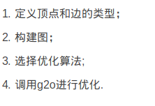
使用G2O拟合曲线,需要将问题抽象成图优化.只需要记住节点为优化变量,边为误差项.步骤:
#include <iostream>
#include <g2o/core/base_vertex.h>
#include <g2o/core/base_unary_edge.h>
#include <g2o/core/block_solver.h>
#include <g2o/core/optimization_algorithm_levenberg.h>
#include <g2o/core/optimization_algorithm_gauss_newton.h>
#include <g2o/core/optimization_algorithm_dogleg.h>
#include <g2o/solvers/dense/linear_solver_dense.h>
#include <Eigen/Core>
#include <opencv2/core/core.hpp>
#include <cmath>
#include <chrono>
using namespace std;

// 曲线模型的顶点,模板参数:优化变量维度和数据类型
class CurveFittingVertex: public g2o::BaseVertex<3, Eigen::Vector3d>
{
public:
    EIGEN_MAKE_ALIGNED_OPERATOR_NEW
    virtual void setToOriginImpl() // 重置
    {
        _estimate << 0,0,0;
    }

    virtual void oplusImpl( const double* update ) // 更新
    {
        _estimate += Eigen::Vector3d(update);
    }
    // 存盘和读盘:留空
    virtual bool read( istream& in ) {}
    virtual bool write( ostream& out ) const {}
};

// 误差模型 模板参数:观测值维度,类型,连接顶点类型
class CurveFittingEdge: public g2o::BaseUnaryEdge<1,double,CurveFittingVertex>
{
public:
    EIGEN_MAKE_ALIGNED_OPERATOR_NEW
    CurveFittingEdge( double x ): BaseUnaryEdge(), _x(x) {}
    // 计算曲线模型误差
    void computeError()
    {
        const CurveFittingVertex* v = static_cast<const CurveFittingVertex*> (_vertices[0]);
        const Eigen::Vector3d abc = v->estimate();
        _error(0,0) = _measurement - std::exp( abc(0,0)*_x*_x + abc(1,0)*_x + abc(2,0) ) ;
    }
    virtual bool read( istream& in ) {}
    virtual bool write( ostream& out ) const {}
public:
    double _x;  // x 值, y 值为 _measurement
};

int main( int argc, char** argv )
{
    double a=1.0, b=2.0, c=1.0;         // 真实参数值
    int N=100;                          // 数据点
    double w_sigma=1.0;                 // 噪声Sigma值
    cv::RNG rng;                        // OpenCV随机数产生器
    double abc[3] = {0,0,0};            // abc参数的估计值

    vector<double> x_data, y_data;      // 数据

    cout<<"generating data: "<<endl;
    for ( int i=0; i<N; i++ )
    {
        double x = i/100.0;
        x_data.push_back ( x );
        y_data.push_back (
            exp ( a*x*x + b*x + c ) + rng.gaussian ( w_sigma )
        );
        cout<<x_data[i]<<" "<<y_data[i]<<endl;
    }

    // 构建图优化,先设定g2o
    typedef g2o::BlockSolver< g2o::BlockSolverTraits<3,1> > Block;  // 每个误差项优化变量维度为3,误差值维度为1
    Block::LinearSolverType* linearSolver = new g2o::LinearSolverDense<Block::PoseMatrixType>(); // 线性方程求解器
    Block* solver_ptr = new Block( linearSolver );      // 矩阵块求解器
    // 梯度下降方法,从GN, LM, DogLeg 中选
    g2o::OptimizationAlgorithmLevenberg* solver = new g2o::OptimizationAlgorithmLevenberg( solver_ptr );
    // g2o::OptimizationAlgorithmGaussNewton* solver = new g2o::OptimizationAlgorithmGaussNewton( solver_ptr );
    // g2o::OptimizationAlgorithmDogleg* solver = new g2o::OptimizationAlgorithmDogleg( solver_ptr );
    g2o::SparseOptimizer optimizer;     // 图模型
    optimizer.setAlgorithm( solver );   // 设置求解器
    optimizer.setVerbose( true );       // 打开调试输出

    // 往图中增加顶点
    CurveFittingVertex* v = new CurveFittingVertex();
    v->setEstimate( Eigen::Vector3d(0,0,0) );
    v->setId(0);
    optimizer.addVertex( v );

    // 往图中增加边
    for ( int i=0; i<N; i++ )
    {
        CurveFittingEdge* edge = new CurveFittingEdge( x_data[i] );
        edge->setId(i);
        edge->setVertex( 0, v );                // 设置连接的顶点
        edge->setMeasurement( y_data[i] );      // 观测数值
        edge->setInformation( Eigen::Matrix<double,1,1>::Identity()*1/(w_sigma*w_sigma) ); // 信息矩阵:协方差矩阵之逆
        optimizer.addEdge( edge );
    }

    // 执行优化
    cout<<"start optimization"<<endl;
    chrono::steady_clock::time_point t1 = chrono::steady_clock::now();
    optimizer.initializeOptimization();
    optimizer.optimize(100);
    chrono::steady_clock::time_point t2 = chrono::steady_clock::now();
    chrono::duration<double> time_used = chrono::duration_cast<chrono::duration<double>>( t2-t1 );
    cout<<"solve time cost = "<<time_used.count()<<" seconds. "<<endl;

    // 输出优化值
    Eigen::Vector3d abc_estimate = v->estimate();
    cout<<"estimated model: "<<abc_estimate.transpose()<<endl;

    return 0;
}
结果如下:
