山东大学机器学习（实验二解读）——逻辑回归和牛顿法

1.梯度下降法

x = load('ex2x.dat');
y = load('ex2y.dat');
m = length(y);
xx = x;
mu = mean(x);
sigma = std(x);
x = (x - mean(x))./std(x); %数据标准化
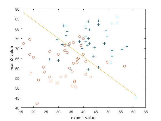
x = [ones(m,1),x] ; xx = [ones(m,1),xx] ;
% find返回满足指定条件的行的索引
pos = find ( y == 1 ) ; neg = find ( y == 0 );
plot (xx( pos , 2 ),xx( pos , 3 ),'+'); 
hold on;
plot (xx( neg , 2 ),xx( neg , 3 ),'o');
xlabel('exam1 value');
ylabel('exam2 value');

MaxIter = 1500;
theta = zeros(size(x(1,:)))'; %初始化theta
e = 1e-6;
alpha = 0.08;
g = @(z) 1./(1+exp(-z)); %定义sigmoid函数
for i = 1:MaxIter
    z = x * theta;
    h = g(z); %逻辑回归模型
    L_theta(i,1) = -(1/m)*sum(y.*log(h)+(1-y).*log(1-h)); %极大对数似然函数
    delta_L = (1/m)*x'*(h-y); %计算梯度   
    %更新 L 和 theta
    if (i > 1) && (abs(L_theta(i,1) - L_theta(i-1,1)) <= e)
        break;
    end
    theta = theta - alpha*delta_L;
    store(i,:) = [theta',L_theta(i,1)];
end

%画出决策边界，因为数据是标准化后的，因此需要还原回去
x_axis = x(:,2)*sigma(1) + mu(1);
y_axis = (-theta(1,1).*x(:,1) - theta(2,1).*x(:,2))/theta(3,1);
y_axis = y_axis*sigma(2) + mu(2);
plot(x_axis, y_axis,'-');
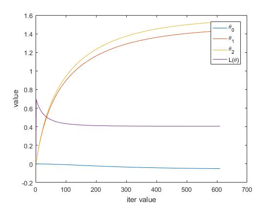
figure;
plot(1:i-1,store,'-');
legend('\theta_0','\theta_1','\theta_2','L{(\theta)}');
xlabel('iter value');
ylabel('value');

假设 $\epsilon = 10 ^ { - 6 }$ 。实现收很慢敛需要多少次迭代？注意，梯度下降算法收敛速度，可能需要很长时间才能达到最小值。

答：610次

收敛后得到的 $\theta$ 值是多少？

$\theta_0 = -0.0506, \ \theta_1 = 1.4305,\ \theta_2 =1.5267$

计算每次迭代过程中的 $L(\theta)$ 和说明 $L(\theta)$ 在梯度下降算法中如何减少。

收敛之后，使用 $\theta$ 的值找出分类问题的决策边界。

测试1的成绩为20分和测试2为80分的学生不被录取的概率是多少？

不被录取的概率为
$P(y=0|x;\theta) = 1 - h_\theta = 1 - g(\theta^Tx) = g(-\theta^Tx)$
先对 $x_1=20,\ x_2 = 80$ 进行标准化
$x_1=(x_1 - \text{mu(1))}/\text{sigma(1)}=-1.7998,\quad x_2=(x_2 - \text{mu(2))}/\text{sigma(2)}=1.2767$
$\theta^T x = −0.0506+1.4305×(−1.7988)+1.5267×1.2767=−0.6746$
最终得到成绩1为20成绩2为80不被录取的概率为
$g(0.6746) = 1/(1+\exp(-0.6746)) = 0.6625$

2. 牛顿法

x = load('ex2x.dat');
y = load('ex2y.dat');
m = length(y);
mu = mean(x);
xx = x;
sigma = std(x);
x = (x - mean(x))./std(x);
x = [ones(m,1),x] ;
n = size(x,2);
% find返回满足指定条件的行的索引
pos = find ( y == 1 ) ; neg = find ( y == 0 ) ;
plot ( xx ( pos , 1 ) , xx ( pos , 2 ) , '+' ) ; 
hold on
plot ( xx ( neg , 1 ) , xx ( neg , 2 ) , ' o ' )
xlabel('exam1 value');
ylabel('exam2 value');
MaxIter = 1500;
theta = zeros(size(x(1,:)))';
e = 1e-6;
H = zeros(n,n);
g = @(x) 1./(1+exp(-x));
for i = 1:MaxIter
    z = x * theta;
    h = g(z); %logistic model
    L_theta(i,1) = -(1/m)*sum(y.*log(h)+(1-y).*log(1-h)); %log likelihood function
    delta_L = (1/m)*x'*(h-y); %calculate gradient   
    %calculate Hessian matrix
    H = (1/m).*x' * diag(h) * diag(1-h) * x;
    %update L and theta
    if (i > 1) && (abs(L_theta(i,1) - L_theta(i-1,1)) <= e )
        break;
    end
    theta = theta - H^(-1)*delta_L;
    store(i,:) = [theta',L_theta(i,1)];
end
x_axis = x(:,2)*sigma(1) + mu(1);
y_axis = (-theta(1,1).*x(:,1) - theta(2,1).*x(:,2))/theta(3,1);
y_axis = y_axis*sigma(2) + mu(2);
plot(x_axis, y_axis,'-');
figure
plot(1:i-1,store,'-');
legend('\theta_0','\theta_1','\theta_2','L{(\theta)}');
xlabel('iter value');
ylabel('value');

当收敛时 $\theta$ 的值是多少？

$\theta_0 = -0.0566, \ \theta_1 = 1.4720,\ \theta_2 =1.5706$

显示牛顿法中 $L$ 是如何减少的？

画出决策边界

测试1的成绩为20分和测试2为80分的学生不被录取的概率是多少？

不被录取的概率为
$P(y=0|x;\theta) = 1 - h_\theta = 1 - g(\theta^Tx) = g(-\theta^Tx)$
先对 $x_1=20,\ x_2 = 80$ 进行标准化
$x_1=(x_1 - \text{mu(1))}/\text{sigma(1)}=-1.7998,\quad x_2=(x_2 - \text{mu(2))}/\text{sigma(2)}=1.2767$
$\theta^T x = −0.0566+1.4720×(−1.7988)+1.5706×1.2767=−0.6993$
最终得到成绩1为20成绩2为80不被录取的概率为
$g(0.6746) = 1/(1+\exp(-0.6993)) = 0.6680$

对比梯度下降法和牛顿法，你学到了什么？

(1)牛顿法：是通过求解目标函数的一阶导数为0时的参数，进而求出目标函数最小值时的参数。
优点：收敛速度很快，而且不需要知道学习率。
海森矩阵的逆在迭代过程中不断减小，可以起到逐步减小步长的效果。
缺点：海森矩阵的逆计算复杂，代价比较大，因此有了拟牛顿法。
(2)梯度下降法：是通过梯度方向和步长，直接求解目标函数的最小值时的参数。
越接近最优值时，步长应该不断减小，否则会在最优值附近来回震荡。
优点：计算简单，实现容易。
缺点：收敛速度比较慢，数据量大还会导致内存不足。

山东大学机器学习（实验二解读）——逻辑回归和牛顿法

1.梯度下降法

2. 牛顿法

猜你喜欢