CNN原理:

受哺乳动物视觉系统的结构启发,人们引入了一个处理图片的强大模型结构,后来发展成了现代卷积网络的基础。所谓卷积引自数学中的卷积运算:
它的意义在于,比如有一段时间内的股票或者其他的测量数据,显然时间离当下越近的数据与结果越相关,作用越大,所以在处理数据时可以采用一种局部加权平均的方法,这就叫卷积,其离散形式为:
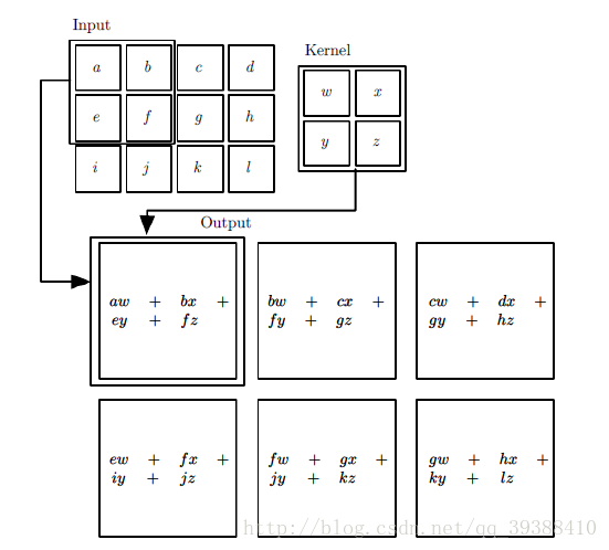
公式中的第一个参数x是输入的数据,第二参数w叫核函数,a表示时间t的时间间隔,而函数的输出可以被叫做特征映射(feature map)。也就是说完成特征映射的过程叫卷积,不过是某一个东西和另一个东西在时间维度上的“叠加”作用。而使用卷积运算的重要作用就是,通过卷积运算,可以使原信号特征增强,并且降低噪音。
卷积神经网络里的卷积层为:
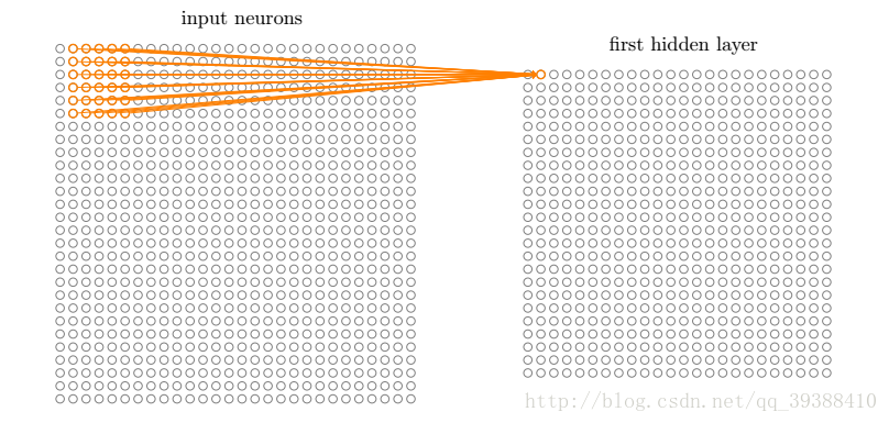
卷积过程采用了稀疏交互(Sparse interactions),参数共享(parameter sharing),等变表示(equivariant representations)三大思想。稀疏交互是利用了局部感受野(local receptive fields),限制了空间的大小,参数共享就是权值共享不但能减少参数数量,还能控制模型规模,增强模型的泛化能力。
如图所示,卷积层的学习输出是:
卷积神经网络里的池化层为:
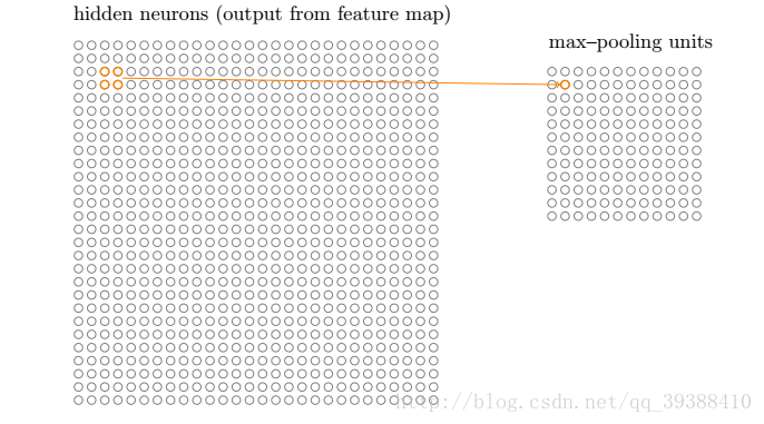
池化层也称亚采样层(Subsampling Layer),简单来说,就是利用其局部相关性,在“采样”数据的同时还保留了有用信息。巧妙的采样还具备局部线性转换不变性(translation invariant),即如果选用连续范围作为池化区域,并且只是池化相同的隐藏单元产生的特征,那么池化单元就具有平移不变性,这意味着即使图像有一个小平移,依然会产生相同的池化特征,这种网络结构对于平移,比例缩放,倾斜,或者共他形式的变形具有高度不变性。而且使用池化可以看作是增加了一个无限强的先验,卷积层学得的函数必须具有对少量平移的不变性,从而增强卷积神经网络的泛化处理能力,预防网络过拟合。而且这样聚合的最直接目的是可以大大降低下一层待处理的数据量,降低了网络的复杂度,减少了参数数量。
池化函数使用某一位置的相邻输出的总计特征来代替网络在该位置的输出,常见的统计特性有最大值、均值、累加和及L2范数等。
如图所示,池化层的输出是:
不过在实践中,有时可能会希望跳过核的一些位置来降低计算开销,由此产生了步幅(stride)。
零填充(zero-padding)以获取低维度:此操作通常用于边界处理。因为有时候卷积核的大小并不一定刚好就被输入数据矩阵的维度大小乘除。因此就可能会出现卷积核不能完全覆盖边界元素的情况,逼迫我们“二选一”。所以这时候就需要在输入矩阵的边缘使用零值进行填充来解决这个问题。而且通过pad操作可以更好的控制特征图的大小。使用零填充的卷积叫做泛卷积(wide convolution),不适用零填充的叫做严格卷积(narrow convolution)。
卷积神经网络里的全连接层为:
全连接层(Fully Connected Layer,简称FC)。“全连接”意味着,前层网络中的所有神经元都与下一层的所有神经元连接。全连接层设计目的在于,它将前面各个层学习到的“分布式特征表示”,映射到样本标记空间,然后利用损失函数来调控学习过程,最后给出对象的分类预测。不同于BP全连接网络的是,卷积神经网络在输出层使用的激活函数不同,比如说它可能会使用Softmax函数,ReLU函数等)。
比如上图网络的具体步骤是:
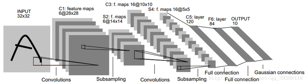
输入为32×32的原图像。
第一层是卷积层C1,经过5×5的的感受野,有6个卷积核,形成6个28×28的特征映射。这层的参数个数为5*5*6+6(偏置项的个数)
第二层是池化层S2,用于实现抽样和池化平均,经过2×2的的感受野,形成6个14×14的特征映射。这层的参数个数为[1(训练得到的参数)+1(训练得到的偏置项)]×6=12
第三层是卷积层C3,与第一层一样,形成16个10×10的特征映射。参数个数为5*5*16+16=416
第四层是池化层S4,与第二层一样,形成16个5×5的特征映射。参数个数为(1+1)*16=32
之后就是120个神经元,64个神经元全连接而成的全连接层,最后得到径向基函数输出结果。
正向传播完成后,将结果与真实值做比较,然后极小化误差反向调整权值矩阵。
TF应用:
CIFAR-10 数据集的分类。
参数说明:
conv2d(input, filter, strides, padding, use_cudnn_on_gpu=None,data_format=None, name=None)
input:输入的数据。格式为张量。[batch, in_height, in_width, in_channels]。
批次,高度,宽度,输入通道数。
filter:卷积核。格式为[filter_height, filter_width, in_channels, out_channels]。
高度,宽度,输入通道数,输出通道数。
strides:步幅
padding:如果是SAME,则保留图像周圈不完全卷积的部分。VALID相反。
use_cudnn_on_gpu:是否使用cudnn加速
max_pool(value, ksize, strides, padding, data_format=“NHWC”, name=None)
value:张量,格式为[batch, height, width, channels]。
批次,高度,宽度,输入通道数。
ksize:窗口大小
strides:步幅
padding:如果是SAME,则保留图像周圈不完全卷积的部分。VALID相反。
import tensorflow as tf
import tensorflow.examples.tutorials.mnist.input_data as input_data

mnist = input_data.read_data_sets("MNIST_data/", one_hot=True)#下载mnist数据集
x = tf.placeholder(tf.float32, [None, 784])
y_actual = tf.placeholder(tf.float32, shape=[None, 10])

#初始化权值 W
def weight_variable(shape):
  initial = tf.truncated_normal(shape, stddev=0.1)
  return tf.Variable(initial)

#初始化偏置项 b
def bias_variable(shape):
  initial = tf.constant(0.1, shape=shape)
  return tf.Variable(initial)

#卷积层
def conv2d(x, W):
  return tf.nn.conv2d(x, W, strides=[1, 1, 1, 1], padding='SAME')

#池化层
def max_pool(x):
  return tf.nn.max_pool(x, ksize=[1, 2, 2, 1],strides=[1, 2, 2, 1], padding='SAME')

#搭建CNN
x_image = tf.reshape(x, [-1,28,28,1])#转换输入数据shape
W_conv1 = weight_variable([5, 5, 1, 32])
b_conv1 = bias_variable([32])
h_conv1 = tf.nn.relu(conv2d(x_image, W_conv1) + b_conv1)#第一个卷积层
h_pool1 = max_pool(h_conv1)#第一个池化层

W_conv2 = weight_variable([5, 5, 32, 64])
b_conv2 = bias_variable([64])
h_conv2 = tf.nn.relu(conv2d(h_pool1, W_conv2) + b_conv2)#第二个卷积层
h_pool2 = max_pool(h_conv2)#第二个池化层

W_fc1 = weight_variable([7 * 7 * 64, 1024])
b_fc1 = bias_variable([1024])
h_pool2_flat = tf.reshape(h_pool2, [-1, 7*7*64])
h_fc1 = tf.nn.relu(tf.matmul(h_pool2_flat, W_fc1) + b_fc1)#第一个全连接层

keep_prob = tf.placeholder("float")
h_fc1_drop = tf.nn.dropout(h_fc1, keep_prob)#dropout

#输出0~9的分类
W_fc2 = weight_variable([1024, 10])
b_fc2 = bias_variable([10])
y_predict=tf.nn.softmax(tf.matmul(h_fc1_drop, W_fc2) + b_fc2)#softmax激活函数

cross_entropy = -tf.reduce_sum(y_actual*tf.log(y_predict))#交叉熵损失函数
train_step = tf.train.GradientDescentOptimizer(1e-3).minimize(cross_entropy)#梯度下降
correct_prediction = tf.equal(tf.argmax(y_predict,1), tf.argmax(y_actual,1))
accuracy = tf.reduce_mean(tf.cast(correct_prediction, "float"))#计算准确度

sess=tf.InteractiveSession()#初始化
sess.run(tf.global_variables_initializer())
for i in range(20000):#内存小的请谨慎设定迭代次数
  batch = mnist.train.next_batch(50)
  if i%100 == 0:#每100次查看进程
    train_acc = accuracy.eval(feed_dict={x:batch[0], y_actual: batch[1], keep_prob: 1.0})
    print ('step %d, training accuracy %g'%(i,train_acc))
    train_step.run(feed_dict={x: batch[0], y_actual: batch[1], keep_prob: 0.5})

test_acc=accuracy.eval(feed_dict={x: mnist.test.images, y_actual: mnist.test.labels, keep_prob: 1.0})
print ("test accuracy %g"%test_acc)
如果用keras实现则是:
from keras import layers
from keras.models import Model

def lenet_5(in_shape=(32,32,1), n_classes=10, opt='sgd'):
   in_layer = layers.Input(in_shape)
   conv1 = layers.Conv2D(filters=20, kernel_size=5,
                         padding='same', activation='relu')(in_layer)
   pool1 = layers.MaxPool2D()(conv1)
   conv2 = layers.Conv2D(filters=50, kernel_size=5,
                         padding='same', activation='relu')(pool1)
   pool2 = layers.MaxPool2D()(conv2)
   flatten = layers.Flatten()(pool2)
   dense1 = layers.Dense(500, activation='relu')(flatten)
   preds = layers.Dense(n_classes, activation='softmax')(dense1)

   model = Model(in_layer, preds)
   model.compile(loss="categorical_crossentropy", optimizer=opt,
               metrics=["accuracy"])
   return model

if __name__ == '__main__':
   model = lenet_5()
   print(model.summary())
卷积只能在同一组进行吗?– Group convolution
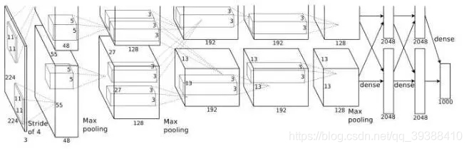
分组卷积最早在AlexNet中出现,由于当时的硬件资源有限,训练AlexNet时卷积操作不能全部放在同一个GPU处理,因此作者把feature maps分给多个GPU分别进行处理,具体架构包括5个卷积层和3个全连接层。这八层也都采用了当时的两个新概念——最大池化和Relu激活来为模型提供优势,最后把多个GPU的结果进行融合。
from keras import layers
from keras.models import Model

def alexnet(in_shape=(227,227,3), n_classes=1000, opt='sgd'):
   in_layer = layers.Input(in_shape)
   conv1 = layers.Conv2D(96, 11, strides=4, activation='relu')(in_layer)
   pool1 = layers.MaxPool2D(3, 2)(conv1)
   conv2 = layers.Conv2D(256, 5, strides=1, padding='same', activation='relu')(pool1)
   pool2 = layers.MaxPool2D(3, 2)(conv2)
   conv3 = layers.Conv2D(384, 3, strides=1, padding='same', activation='relu')(pool2)
   conv4 = layers.Conv2D(256, 3, strides=1, padding='same', activation='relu')(conv3)
   pool3 = layers.MaxPool2D(3, 2)(conv4)
   flattened = layers.Flatten()(pool3)
   dense1 = layers.Dense(4096, activation='relu')(flattened)
   drop1 = layers.Dropout(0.5)(dense1)
   dense2 = layers.Dense(4096, activation='relu')(drop1)
   drop2 = layers.Dropout(0.5)(dense2)
   preds = layers.Dense(n_classes, activation='softmax')(drop2)

   model = Model(in_layer, preds)
   model.compile(loss="categorical_crossentropy", optimizer=opt,
               metrics=["accuracy"])
   return model

if __name__ == '__main__':
   model = alexnet()
   print(model.summary())
卷积核一定越大越好?– 3×3卷积核
AlexNet中用到了一些非常大的卷积核,比如11×11、5×5卷积核,之前人们的观念是,卷积核越大,receptive field(感受野)越大,看到的图片信息越多,因此获得的特征越好。但是大的卷积核会导致计算量的暴增,不利于模型深度的增加,计算性能也会降低。于是在VGG(最早使用,代码如下)、Inception网络中,利用2个3×3卷积核的组合比1个5×5卷积核的效果更佳,同时参数量(3×3×2+1 VS 5×5×1+1)被降低,因此后来3×3卷积核被广泛应用在各种模型中。
from keras import layers
from keras.models import Model, Sequential

from functools import partial

conv3 = partial(layers.Conv2D,
               kernel_size=3,
               strides=1,
               padding='same',
               activation='relu')

def block(in_tensor, filters, n_convs):
   conv_block = in_tensor
   for _ in range(n_convs):
       conv_block = conv3(filters=filters)(conv_block)
   return conv_block

def _vgg(in_shape=(227,227,3),
        n_classes=1000,
        opt='sgd',
        n_stages_per_blocks=[2, 2, 3, 3, 3]):
   in_layer = layers.Input(in_shape)

   block1 = block(in_layer, 64, n_stages_per_blocks[0])
   pool1 = layers.MaxPool2D()(block1)
   block2 = block(pool1, 128, n_stages_per_blocks[1])
   pool2 = layers.MaxPool2D()(block2)
   block3 = block(pool2, 256, n_stages_per_blocks[2])
   pool3 = layers.MaxPool2D()(block3)
   block4 = block(pool3, 512, n_stages_per_blocks[3])
   pool4 = layers.MaxPool2D()(block4)
   block5 = block(pool4, 512, n_stages_per_blocks[4])
   pool5 = layers.MaxPool2D()(block5)
   flattened = layers.GlobalAvgPool2D()(pool5)

   dense1 = layers.Dense(4096, activation='relu')(flattened)
   dense2 = layers.Dense(4096, activation='relu')(dense1)
   preds = layers.Dense(1000, activation='softmax')(dense2)

   model = Model(in_layer, preds)
   model.compile(loss="categorical_crossentropy", optimizer=opt,
               metrics=["accuracy"])
   return model

def vgg16(in_shape=(227,227,3), n_classes=1000, opt='sgd'):
   return _vgg(in_shape, n_classes, opt)

def vgg19(in_shape=(227,227,3), n_classes=1000, opt='sgd'):
   return _vgg(in_shape, n_classes, opt, [2, 2, 4, 4, 4])

if __name__ == '__main__':
   model = vgg19()
   print(model.summary())
每层卷积只能用一种尺寸的卷积核?– Inception结构
传统的层叠式网络,基本上都是一个个卷积层的堆叠,每层只用一个尺寸的卷积核,例如VGG结构中使用了大量的3×3卷积层。事实上,同一层feature map可以分别使用多个不同尺寸的卷积核,以获得不同尺度的特征,再把这些特征结合起来,得到的特征往往比使用单一卷积核的要好,谷歌的GoogleNet。但是同样的,参数量加大,计算量会暴增。
怎样才能减少卷积层参数量?– Bottleneck
Inception结构中加入了一些1×1的卷积核降维!
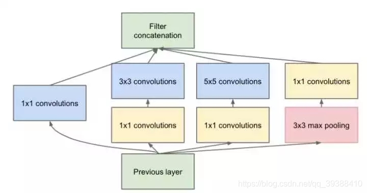
如果一个n维的直接进过3x3卷积,将会有nx3x3xn的参数(若输出也为n维),如果在前后各加一层1x1,则会有n×1×1×(n/4) + (n/4)×3×3×(n/4) + (n/4)×1×1×n,将会大大减少参数。所以1×1卷积核也被认为是影响深远的操作,往后大型的网络为了降低参数量都会应用上1×1卷积核。
GoogLeNet/Inception 的 架构实现如下:
from keras import layers
from keras.models import Model

from functools import partial

conv1x1 = partial(layers.Conv2D, kernel_size=1, activation='relu')
conv3x3 = partial(layers.Conv2D, kernel_size=3, padding='same', activation='relu')
conv5x5 = partial(layers.Conv2D, kernel_size=5, padding='same', activation='relu')

def inception_module(in_tensor, c1, c3_1, c3, c5_1, c5, pp):
   conv1 = conv1x1(c1)(in_tensor)

   conv3_1 = conv1x1(c3_1)(in_tensor)
   conv3 = conv3x3(c3)(conv3_1)

   conv5_1 = conv1x1(c5_1)(in_tensor)
   conv5 = conv5x5(c5)(conv5_1)

   pool_conv = conv1x1(pp)(in_tensor)
   pool = layers.MaxPool2D(3, strides=1, padding='same')(pool_conv)

   merged = layers.Concatenate(axis=-1)([conv1, conv3, conv5, pool])
   return merged

def aux_clf(in_tensor):
   avg_pool = layers.AvgPool2D(5, 3)(in_tensor)
   conv = conv1x1(128)(avg_pool)
   flattened = layers.Flatten()(conv)
   dense = layers.Dense(1024, activation='relu')(flattened)
   dropout = layers.Dropout(0.7)(dense)
   out = layers.Dense(1000, activation='softmax')(dropout)
   return out

def inception_net(in_shape=(224,224,3), n_classes=1000, opt='sgd'):
   in_layer = layers.Input(in_shape)

   conv1 = layers.Conv2D(64, 7, strides=2, activation='relu', padding='same')(in_layer)
   pad1 = layers.ZeroPadding2D()(conv1)
   pool1 = layers.MaxPool2D(3, 2)(pad1)
   conv2_1 = conv1x1(64)(pool1)
   conv2_2 = conv3x3(192)(conv2_1)
   pad2 = layers.ZeroPadding2D()(conv2_2)
   pool2 = layers.MaxPool2D(3, 2)(pad2)

   inception3a = inception_module(pool2, 64, 96, 128, 16, 32, 32)
   inception3b = inception_module(inception3a, 128, 128, 192, 32, 96, 64)
   pad3 = layers.ZeroPadding2D()(inception3b)
   pool3 = layers.MaxPool2D(3, 2)(pad3)

   inception4a = inception_module(pool3, 192, 96, 208, 16, 48, 64)
   inception4b = inception_module(inception4a, 160, 112, 224, 24, 64, 64)
   inception4c = inception_module(inception4b, 128, 128, 256, 24, 64, 64)
   inception4d = inception_module(inception4c, 112, 144, 288, 32, 48, 64)
   inception4e = inception_module(inception4d, 256, 160, 320, 32, 128, 128)
   pad4 = layers.ZeroPadding2D()(inception4e)
   pool4 = layers.MaxPool2D(3, 2)(pad4)

   aux_clf1 = aux_clf(inception4a)
   aux_clf2 = aux_clf(inception4d)

   inception5a = inception_module(pool4, 256, 160, 320, 32, 128, 128)
   inception5b = inception_module(inception5a, 384, 192, 384, 48, 128, 128)
   pad5 = layers.ZeroPadding2D()(inception5b)
   pool5 = layers.MaxPool2D(3, 2)(pad5)

   avg_pool = layers.GlobalAvgPool2D()(pool5)
   dropout = layers.Dropout(0.4)(avg_pool)
   preds = layers.Dense(1000, activation='softmax')(dropout)

   model = Model(in_layer, [preds, aux_clf1, aux_clf2])
   model.compile(loss="categorical_crossentropy", optimizer=opt,
               metrics=["accuracy"])
   return model

if __name__ == '__main__':
   model = inception_net()
   print(model.summary())
越深的网络就越难训练吗?– Resnet残差网络
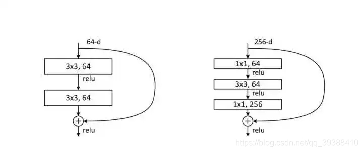
传统的卷积层层叠网络会遇到一个问题,当层数加深时,网络的表现越来越差,很大程度上的原因是因为当层数加深时,梯度消失得越来越严重,以至于反向传播很难训练到浅层的网络。直接映射是很难学习的,所以不去学习网络输出层与输入层间的映射,而是学习它们之间的差异——残差。下面是残差网络的实现:
from keras import layers
from keras.models import Model

def _after_conv(in_tensor):
   norm = layers.BatchNormalization()(in_tensor)
   return layers.Activation('relu')(norm)

def conv1(in_tensor, filters):
   conv = layers.Conv2D(filters, kernel_size=1, strides=1)(in_tensor)
   return _after_conv(conv)

def conv1_downsample(in_tensor, filters):
   conv = layers.Conv2D(filters, kernel_size=1, strides=2)(in_tensor)
   return _after_conv(conv)

def conv3(in_tensor, filters):
   conv = layers.Conv2D(filters, kernel_size=3, strides=1, padding='same')(in_tensor)
   return _after_conv(conv)

def conv3_downsample(in_tensor, filters):
   conv = layers.Conv2D(filters, kernel_size=3, strides=2, padding='same')(in_tensor)
   return _after_conv(conv)

def resnet_block_wo_bottlneck(in_tensor, filters, downsample=False):
   if downsample:
       conv1_rb = conv3_downsample(in_tensor, filters)
   else:
       conv1_rb = conv3(in_tensor, filters)
   conv2_rb = conv3(conv1_rb, filters)

   if downsample:
       in_tensor = conv1_downsample(in_tensor, filters)
   result = layers.Add()([conv2_rb, in_tensor])

   return layers.Activation('relu')(result)

def resnet_block_w_bottlneck(in_tensor,
                            filters,
                            downsample=False,
                            change_channels=False):
   if downsample:
       conv1_rb = conv1_downsample(in_tensor, int(filters/4))
   else:
       conv1_rb = conv1(in_tensor, int(filters/4))
   conv2_rb = conv3(conv1_rb, int(filters/4))
   conv3_rb = conv1(conv2_rb, filters)

   if downsample:
       in_tensor = conv1_downsample(in_tensor, filters)
   elif change_channels:
       in_tensor = conv1(in_tensor, filters)
   result = layers.Add()([conv3_rb, in_tensor])

   return result

def _pre_res_blocks(in_tensor):
   conv = layers.Conv2D(64, 7, strides=2, padding='same')(in_tensor)
   conv = _after_conv(conv)
   pool = layers.MaxPool2D(3, 2, padding='same')(conv)
   return pool

def _post_res_blocks(in_tensor, n_classes):
   pool = layers.GlobalAvgPool2D()(in_tensor)
   preds = layers.Dense(n_classes, activation='softmax')(pool)
   return preds

def convx_wo_bottleneck(in_tensor, filters, n_times, downsample_1=False):
   res = in_tensor
   for i in range(n_times):
       if i == 0:
           res = resnet_block_wo_bottlneck(res, filters, downsample_1)
       else:
           res = resnet_block_wo_bottlneck(res, filters)
   return res

def convx_w_bottleneck(in_tensor, filters, n_times, downsample_1=False):
   res = in_tensor
   for i in range(n_times):
       if i == 0:
           res = resnet_block_w_bottlneck(res, filters, downsample_1, not downsample_1)
       else:
           res = resnet_block_w_bottlneck(res, filters)
   return res

def _resnet(in_shape=(224,224,3),
           n_classes=1000,
           opt='sgd',
           convx=[64, 128, 256, 512],
           n_convx=[2, 2, 2, 2],
           convx_fn=convx_wo_bottleneck):
   in_layer = layers.Input(in_shape)

   downsampled = _pre_res_blocks(in_layer)

   conv2x = convx_fn(downsampled, convx[0], n_convx[0])
   conv3x = convx_fn(conv2x, convx[1], n_convx[1], True)
   conv4x = convx_fn(conv3x, convx[2], n_convx[2], True)
   conv5x = convx_fn(conv4x, convx[3], n_convx[3], True)

   preds = _post_res_blocks(conv5x, n_classes)

   model = Model(in_layer, preds)
   model.compile(loss="categorical_crossentropy", optimizer=opt,
               metrics=["accuracy"])
   return model

def resnet18(in_shape=(224,224,3), n_classes=1000, opt='sgd'):
   return _resnet(in_shape, n_classes, opt)

def resnet34(in_shape=(224,224,3), n_classes=1000, opt='sgd'):
   return _resnet(in_shape,
                 n_classes,
                 opt,
                 n_convx=[3, 4, 6, 3])

def resnet50(in_shape=(224,224,3), n_classes=1000, opt='sgd'):
   return _resnet(in_shape,
                 n_classes,
                 opt,
                 [256, 512, 1024, 2048],
                 [3, 4, 6, 3],
                 convx_w_bottleneck)

def resnet101(in_shape=(224,224,3), n_classes=1000, opt='sgd'):
   return _resnet(in_shape,
                 n_classes,
                 opt,
                 [256, 512, 1024, 2048],
                 [3, 4, 23, 3],
                 convx_w_bottleneck)

def resnet152(in_shape=(224,224,3), n_classes=1000, opt='sgd'):
   return _resnet(in_shape,
                 n_classes,
                 opt,
                 [256, 512, 1024, 2048],
                 [3, 8, 36, 3],
                 convx_w_bottleneck)

if __name__ == '__main__':
   model = resnet50()
   print(model.summary())
卷积操作时必须同时考虑通道和区域吗?– DepthWise操作
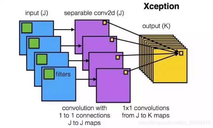
DW:首先对每一个通道进行各自的卷积操作,有多少个通道就有多少个过滤器。得到新的通道feature maps之后,这时再对这批新的通道feature maps进行标准的1×1跨通道卷积操作。
如果直接一个3×3×256的卷积核,参数量为:3×3×3×256(通道数为3,输出为256),DW的参数量为:3×3×3 + 3×1×1×256,又再次大大减少了参数量。
分组卷积能否对通道进行随机分组?– ShuffleNet
通道间的特征都是平等的吗? – SEnet
能否让固定大小的卷积核看到更大范围的区域?– Dilated convolution
卷积核大小依然是3×3,但是每个卷积点之间有1个空洞,也就是在绿色7×7区域里面,只有9个红色点位置作了卷积处理,其余点权重为0。这样即使卷积核大小不变,但它看到的区域变得更大了。
卷积核形状一定是矩形吗?– Deformable convolution 可变形卷积核
直接在原来的过滤器前面再加一层过滤器,这层过滤器学习的是下一层卷积核的位置偏移量(offset)。变形的卷积核能让它只看感兴趣的图像区域 ,这样识别出来的特征更佳。
主要参考:
bengio deep learning
深度思考·DeepThinking
Faisal Shahbaz Five Powerful CNN Architectures