版权声明:本文为博主原创文章,未经博主允许不得转载。 https://blog.csdn.net/weixin_42432468
学习心得:
1、每周的视频课程看一到两遍
2、做笔记
3、做每周的作业练习,这个里面的含金量非常高。先根据notebook过一遍,掌握后一定要自己敲一遍,这样以后用起来才能得心应手。
1、Load Dataset
1.1、观察数据
1.2、数据处理(归一化、去极值、缺失值处理等)
2、构建优化流图
2.1、Create Placeholders
2.2、Initialize Parameters
2.3、Forward Propagation
2.4、Compute Cost
2.5、Optimizer
3、初始化变量
tf.global_variables_initializer()
4、优化过程实例化
5、画图展示cost变化趋势
6、Accuracy构建流图和实例化
import math
import numpy as np
import h5py
import matplotlib.pyplot as plt
import scipy
from PIL import Image
from scipy import ndimage
import tensorflow as tf
from tensorflow.python.framework import ops
from cnn_utils_yhd import *

%matplotlib inline
np.random.seed(1)
1、Load Dataset
1.1、观察数据
# Loading the data (signs)
X_train_orig, Y_train_orig, X_test_orig, Y_test_orig, classes = load_dataset()

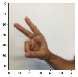
index = 6
plt.imshow(X_train_orig[index])
print ('y = ',np.squeeze(Y_train_orig[:,index]))
y = 2
1.2、数据处理(归一化、去极值、缺失值处理等)
'''
numpy.eye(N,M=None, k=0, dtype=<type 'float'>)
关注第一个第三个参数就行了
第一个参数:输出方阵(行数=列数)的规模,即行数或列数
第三个参数:默认情况下输出的是对角线全“1”,其余全“0”的方阵,如果k为正整数,则在右上方第k条对角线全“1”其余全“0”,k为负整数则在左下方第k条对角线全“1”其余全“0”。

'''
a = np.eye(2,dtype=int)
print (a)
[[1 0]
 [0 1]]
def convert_to_one_hot(Y, C):
#     Y = np.eye(C)[Y.reshape(-1)].T
    '函数分解为下面三步'
    a = np.eye(C)
    a = a[Y.reshape(-1)]   # 这一步怎么理解?
    Y = a.T
    return Y
# test convert_to_one_hot function
np.random.seed(1)
Y = np.random.randint(0,6,7).reshape(1,7)
print (Y)

Y = convert_to_one_hot(Y,6)
print (Y)
[[5 3 4 0 1 3 5]]
[[0. 0. 0. 1. 0. 0. 0.]
 [0. 0. 0. 0. 1. 0. 0.]
 [0. 0. 0. 0. 0. 0. 0.]
 [0. 1. 0. 0. 0. 1. 0.]
 [0. 0. 1. 0. 0. 0. 0.]
 [1. 0. 0. 0. 0. 0. 1.]]
X_train = X_train_orig/255
X_test = X_test_orig/255
Y_train = convert_to_one_hot(Y_train_orig,6).T
Y_test = convert_to_one_hot(Y_test_orig,6).T

print ("number of training examples = " + str(X_train.shape[0]))
print ("number of test examples = " + str(X_test.shape[0]))
print ("X_train shape: " + str(X_train.shape))
print ("Y_train shape: " + str(Y_train.shape))
print ("X_test shape: " + str(X_test.shape))
print ("Y_test shape: " + str(Y_test.shape))
number of training examples = 1080
number of test examples = 120
X_train shape: (1080, 64, 64, 3)
Y_train shape: (1080, 6)
X_test shape: (120, 64, 64, 3)
Y_test shape: (120, 6)
2、构建优化流图
2.1、Create Placeholders
def create_placeholders(n_H0,n_W0,n_C0,n_y):
    X = tf.placeholder(tf.float32,shape=[None,n_H0,n_W0,n_C0])
    Y = tf.placeholder(tf.float32,shape=[None,n_y])
    return X,Y
# test create_placeholders function
X, Y = create_placeholders(64, 64, 3, 6)
print ("X = " + str(X))
print ("Y = " + str(Y))
X = Tensor("Placeholder_2:0", shape=(?, 64, 64, 3), dtype=float32)
Y = Tensor("Placeholder_3:0", shape=(?, 6), dtype=float32)
2.2、Initialize Parameters
def initialize_parameters():
    tf.set_random_seed(1)
    W1 = tf.get_variable('W1',[4,4,3,8],initializer=tf.contrib.layers.xavier_initializer(seed=0))
    W2 = tf.get_variable('W2',[2,2,8,16],initializer=tf.contrib.layers.xavier_initializer(seed=0))
    parameters = {"W1": W1,
                  "W2": W2}
    return parameters
# test initialize_parameters function
tf.reset_default_graph()
with tf.Session() as sess_test:
    parameters = initialize_parameters()
    init = tf.global_variables_initializer()
    sess_test.run(init)
    print ('W1 = ',parameters['W1'].eval()[1,1,1])
    print ('W2 = ',parameters['W2'].eval()[1,1,1])
W1 =  [ 0.00131723  0.1417614  -0.04434952  0.09197326  0.14984085 -0.03514394
 -0.06847463  0.05245192]
W2 =  [-0.08566415  0.17750949  0.11974221  0.16773748 -0.0830943  -0.08058
 -0.00577033 -0.14643836  0.24162132 -0.05857408 -0.19055021  0.1345228
 -0.22779644 -0.1601823  -0.16117483 -0.10286498]
2.3、Forward Propagation
def forward_propagation(X,parameters):
    '''
    X -> Z1 -> A1 -> P1 -> Z2 -> A2 -> P2 ->Z3
    '''
    W1 = parameters['W1']/np.sqrt(2)  # 为什么/np.sqrt(2)效果会更好?
    W2 = parameters['W2']/np.sqrt(2)

    Z1 = tf.nn.conv2d(X,W1,strides=[1,1,1,1],padding='SAME')
    A1 = tf.nn.relu(Z1)
    P1 = tf.nn.max_pool(A1,ksize=[1,8,8,1],strides=[1,8,8,1],padding='SAME')

    Z2 = tf.nn.conv2d(P1,W2,strides=[1,1,1,1],padding='SAME')
    A2 = tf.nn.relu(Z2)
    P2 = tf.nn.max_pool(A2,ksize=[1,4,4,1],strides=[1,4,4,1],padding='SAME')

    P2 = tf.contrib.layers.flatten(P2)

    Z3 = tf.contrib.layers.fully_connected(P2,6,activation_fn=None)

    return Z3
# test forward_propagation function
tf.reset_default_graph()

with tf.Session() as sess:
    np.random.seed(1)
    X,Y = create_placeholders(64,64,3,6)
    parameters = initialize_parameters()
    Z3 = forward_propagation(X,parameters)
    init = tf.global_variables_initializer()
    sess.run(init)
    a = sess.run(Z3, feed_dict={X: np.random.randn(2,64,64,3), Y: np.random.randn(2,6)})
    print ('Z3 = ',a)

    '''
    此处跟课后答案有些不同,是因为我们使用的TensorFlow版本不同而已
    '''
Z3 =  [[ 0.63031745 -0.9877705  -0.4421346   0.05680432  0.5849418   0.12013616]
 [ 0.43707377 -1.0388098  -0.5433439   0.0261174   0.57343066  0.02666192]]
2.4、Compute Cost
def compute_cost(Z3,Y):
    cost = tf.reduce_mean(tf.nn.softmax_cross_entropy_with_logits(logits=Z3,labels=Y))
    return cost
# test copute_cost function
tf.reset_default_graph()

with tf.Session() as sess:
    np.random.seed(1)
    X,Y = create_placeholders(64,64,3,6)
    parameters = initialize_parameters()
    Z3 = forward_propagation(X,parameters)
    cost = compute_cost(Z3,Y)
    init = tf.global_variables_initializer()
    sess.run(init)
    a = sess.run(cost,feed_dict={X: np.random.randn(4,64,64,3), Y: np.random.randn(4,6)})
    print ('cost =',a)
cost = 2.2026021
2.5、Optimizer
3、初始化变量
tf.global_variables_initializer()
4、优化过程实例化
5、画图展示cost变化趋势
6、Accuracy构建流图和实例化
def random_mini_batches(X, Y, mini_batch_size = 64, seed = 0):
    """
    Creates a list of random minibatches from (X, Y)

    Arguments:
    X -- input data, of shape (input size, number of examples) (m, Hi, Wi, Ci)
    Y -- true "label" vector (containing 0 if cat, 1 if non-cat), of shape (1, number of examples) (m, n_y)
    mini_batch_size - size of the mini-batches, integer
    seed -- this is only for the purpose of grading, so that you're "random minibatches are the same as ours.

    Returns:
    mini_batches -- list of synchronous (mini_batch_X, mini_batch_Y)
    """

    m = X.shape[0]                  # number of training examples
    mini_batches = []
    np.random.seed(seed)

    # Step 1: Shuffle (X, Y)
    permutation = list(np.random.permutation(m))
    shuffled_X = X[permutation,:,:,:]
    shuffled_Y = Y[permutation,:]

    # Step 2: Partition (shuffled_X, shuffled_Y). Minus the end case.
    num_complete_minibatches = math.floor(m/mini_batch_size) # number of mini batches of size mini_batch_size in your partitionning
    for k in range(0, num_complete_minibatches):
        mini_batch_X = shuffled_X[k * mini_batch_size : k * mini_batch_size + mini_batch_size,:,:,:]
        mini_batch_Y = shuffled_Y[k * mini_batch_size : k * mini_batch_size + mini_batch_size,:]
        mini_batch = (mini_batch_X, mini_batch_Y)
        mini_batches.append(mini_batch)

    # Handling the end case (last mini-batch < mini_batch_size)
    if m % mini_batch_size != 0:
        mini_batch_X = shuffled_X[num_complete_minibatches * mini_batch_size : m,:,:,:]
        mini_batch_Y = shuffled_Y[num_complete_minibatches * mini_batch_size : m,:]
        mini_batch = (mini_batch_X, mini_batch_Y)
        mini_batches.append(mini_batch)

    return mini_batches
# test  random_mini_batches function
minibatches_test = random_mini_batches(X_train, Y_train, 64, 1)
minibatch_test = minibatches_test[1]
(X_test,Y_test) = minibatch_test
print (X_test[1,1,1])
[0.90980392 0.87843137 0.85098039]
def model(X_train, Y_train, X_test, Y_test, learning_rate = 0.009,
num_epochs = 100, minibatch_size = 64, print_cost = True):
tf.reset_default_graph()
tf.set_random_seed(1)
seed = 3
(m,n_H0,n_W0,n_C0) = X_train.shape
n_y = Y_train.shape[1]
costs = []
X,Y = create_placeholders(n_H0,n_W0,n_C0,n_y)
parameters = initialize_parameters()
Z3 = forward_propagation(X,parameters)
cost = compute_cost(Z3,Y)
# 2.5、Optimizer
optimizer = tf.train.AdamOptimizer(learning_rate=learning_rate).minimize(cost)
# 3、初始化变量
init = tf.global_variables_initializer()
# 4、优化过程实例化流图
with tf.Session() as sess:
sess.run(init)
for epoch in range(num_epochs):
minibatch_cost = 0
num_minibatches = int(m/minibatch_size)
seed = seed +1
minibatches = random_mini_batches(X_train, Y_train, minibatch_size, seed)
for minibatch in minibatches:
(minibatch_X,minibatch_Y) = minibatch
_,temp_cost = sess.run([optimizer,cost],feed_dict={X:minibatch_X,Y: minibatch_Y})
minibatch_cost +=temp_cost/num_minibatches
if print_cost == True and epoch%5 ==0:
print('cost after epoch %i:%f'%(epoch,minibatch_cost))
if print_cost == True and epoch%1 == 0:
costs.append(minibatch_cost)
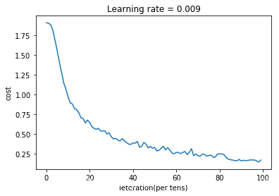
# 5、画图展示cost变化趋势
plt.plot(np.squeeze(costs))
plt.ylabel('cost')
plt.xlabel('ieteration(per tens)')
plt.title('Learning rate = '+ str(learning_rate))
plt.show()
# 6、Accuracy构建流图和实例化
# 6.1 构建Accuracy流图
predict_op = tf.argmax(Z3,1)
'''
tf.argmax(vector, 1):返回的是vector中的最大值的索引号,
如果vector是一个向量,那就返回一个值,如果是一个矩阵,那就返回一个向量,
这个向量的每一个维度都是相对应矩阵行的最大值元素的索引号
'''
correct_prediction = tf.equal(predict_op,tf.argmax(Y,1))
accuracy = tf.reduce_mean(tf.cast(correct_prediction,'float'))
'''
tf.reduce_mean(input_tensor, axis=None, keep_dims=False, name=None, reduction_indices=None)
根据给出的axis在input_tensor上求平均值。除非keep_dims为真,axis中的每个的张量秩会减少1。如果keep_dims为真,
求平均值的维度的长度都会保持为1.如果不设置axis,所有维度上的元素都会被求平均值,并且只会返回一个只有一个元素的张量。
'''
'''
cast(x,dtype,name=None)
将x的数据格式转化成dtype.例如,原来x的数据格式是bool,
那么将其转化成float以后,就能够将其转化成0和1的序列
'''
# 6.2 Accuracy流图实例化
train_accuracy = accuracy.eval(feed_dict={X: X_train,Y: Y_train})
test_accuracy = accuracy.eval(feed_dict={X: X_test,Y: Y_test})
'''
Tensor.eval(feed_dict=None, session=None):
作用: 在一个Seesion里面“评估”tensor的值(其实就是计算),首先执行之前的所有必要的操作来产生这个计算这个tensor
需要的输入,然后通过这些输入产生这个tensor。在激发tensor.eval()这个函数之前,tensor的图必须已经投入到session
里面,或者一个默认的session是有效的,或者显式指定session.
参数:feed_dict:一个字典,用来表示tensor被feed的值(联系placeholder一起看)
session:(可选) 用来计算(evaluate)这个tensor的session.要是没有指定的话,那么就会使用默认的session。
返回: 表示“计算”结果值的numpy ndarray
'''
print ('Train Accuracy :',train_accuracy)
print ('Test Accuracy :',test_accuracy)
return train_accuracy,test_accuracy,parameters
_, _, parameters = model(X_train, Y_train, X_test, Y_test)
cost after epoch 0:1.906084
cost after epoch 5:1.554747
cost after epoch 10:0.971529
cost after epoch 15:0.767831
cost after epoch 20:0.648505
cost after epoch 25:0.536914
cost after epoch 30:0.463869
cost after epoch 35:0.440091
cost after epoch 40:0.385492
cost after epoch 45:0.392317
cost after epoch 50:0.327990
cost after epoch 55:0.296814
cost after epoch 60:0.266418
cost after epoch 65:0.238285
cost after epoch 70:0.224210
cost after epoch 75:0.223669
cost after epoch 80:0.248607
cost after epoch 85:0.173516
cost after epoch 90:0.158102
cost after epoch 95:0.170466
Train Accuracy : 0.94166666
Test Accuracy : 0.953125
# 为什么test Accuracy不一样呢?