线性回归的改进-岭回归
文章源代码下载地址:波士顿房价岭回归正则化预测代码实现
1.API
- sklearn.linear_model.Ridge(alpha=1.0, fit_intercept=True,solver=“auto”, normalize=False)
- 具有l2正则化的线性回归
- alpha:正则化力度,也叫 λ
- λ取值:0~1 1~10
- solver:会根据数据自动选择优化方法
- sag:如果数据集、特征都比较大,选择该随机梯度下降优化
- normalize:数据是否进行标准化
- normalize=False:可以在fit之前调用preprocessing.StandardScaler标准化数据
- Ridge.coef_:回归权重
- Ridge.intercept_:回归偏置
Ridge方法相当于SGDRegressor(penalty=‘l2’, loss=“squared_loss”),只不过SGDRegressor实现了一个普通的随机梯度下降学习,推荐使用Ridge(实现了SAG)
- sklearn.linear_model.RidgeCV(_BaseRidgeCV, RegressorMixin)
- 具有l2正则化的线性回归,可以进行交叉验证
- coef_:回归系数
class _BaseRidgeCV(LinearModel):
    def __init__(self, alphas=(0.1, 1.0, 10.0),
                 fit_intercept=True, normalize=False,scoring=None,
                 cv=None, gcv_mode=None,
                 store_cv_values=False):
2.观察正则化程度的变化,对结果的影响?
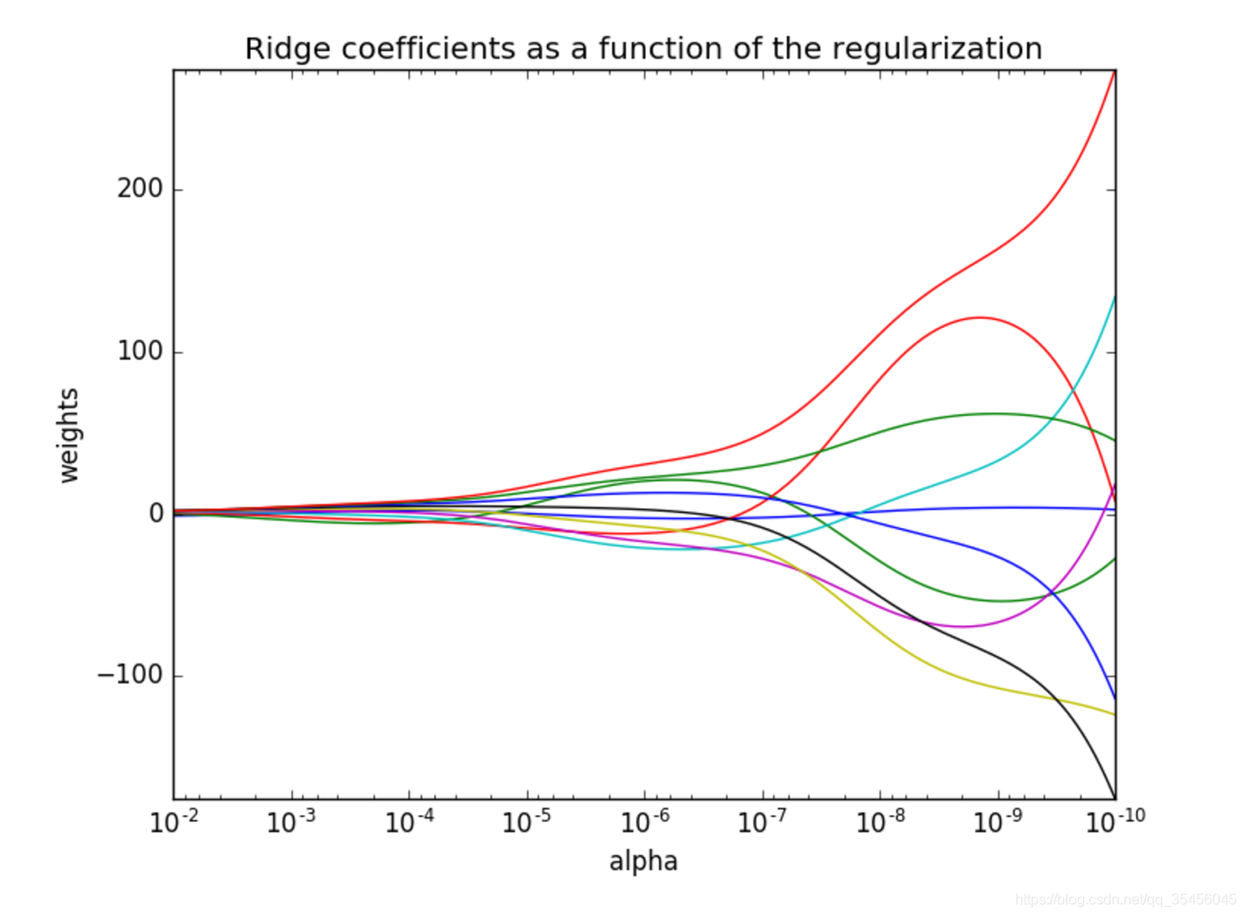
- 正则化力度越大,权重系数会越小(聚集在0附近了)
- 正则化力度越小,权重系数会越大
3.波士顿房价正则化预测代码
#要用到的包
from sklearn.datasets import load_boston
from sklearn.model_selection import train_test_split
from sklearn.preprocessing import StandardScaler
from sklearn.linear_model import LinearRegression
from sklearn.metrics import mean_squared_error
from sklearn.linear_model import SGDRegressor
from sklearn.linear_model import Ridge#导入岭回归
# 1.获取数据 laod_boston bunch字典
data = load_boston()

# 2.数据集划分 数据的基本处理
x_train, x_test, y_train, y_test = train_test_split(data.data, data.target, random_state=22)

# 3.特征工程-标准化
transfer = StandardScaler()
x_train = transfer.fit_transform(x_train)
x_test = transfer.fit_transform(x_test)

# 4.机器学习-线性回归(岭回归)【重要】
# 4.1 创建模型 实例化估计器
estimator = Ridge(alpha=1)#(alpha表示正则的程度)
# 4.2 训练模型 fit 正规方程计算得到最优可训练参数
estimator.fit(x_train, y_train)

# 5.模型评估
# 5.1 获取系数等值
y_predict = estimator.predict(x_test)
print("预测值为:\n", y_predict)
print("模型中的系数为:\n", estimator.coef_)
print("模型中的偏置为:\n", estimator.intercept_)

# 5.2 评价
# 均方误差
error = mean_squared_error(y_test, y_predict)
print("误差为:\n", error)
4.结果
预测值为:
 [28.14336439 31.29120593 20.54384341 31.45949883 19.05713232 18.25154031
 20.59333004 18.46668579 18.49439324 32.90278303 20.39074387 27.19391547
 14.82896742 19.22647169 36.99680592 18.30216415  7.77234952 17.59204777
 30.20233488 23.61819202 18.13165677 33.80976641 28.45514573 16.97450477
 34.72448519 26.19876013 34.77528305 26.63056236 18.62636595 13.34630747
 30.34386216 14.5911294  37.18589518  8.96603866 15.1046276  16.0870778
  7.2410686  19.13817477 39.5390249  28.27770546 24.63218813 16.74118324
 37.8401846   5.70041018 21.17142785 24.60567485 18.90535427 19.95506965
 15.19437924 26.28324334  7.54840338 27.10725806 29.18271353 16.27866225
  7.9813597  35.42054763 32.2845617  20.95634259 16.43407021 20.88411873
 22.93442975 23.58724813 19.3655118  38.2810092  23.98858525 18.95166781
 12.62360991  6.12834839 41.45200493 21.09795707 16.19808353 21.5210458
 40.71914496 20.54014744 36.78495192 27.02863306 19.9217193  19.64062326
 24.60418297 21.26677099 30.94032672 19.33770303 22.30888436 31.07881055
 26.39477737 20.24104002 28.79548502 20.86317185 26.04545844 19.2573741
 24.92683599 22.29008698 18.92825484 18.92207977 14.04840276 17.41630198
 24.16632188 15.83303972 20.04416558 26.5192807  20.10159263 17.02240369
 23.84898152 22.82854834 20.89047727 36.1141591  14.72135442 20.67674724
 32.4387071  33.1767914  19.81979219 26.46158288 20.97213033 16.46431333
 20.7661367  20.59296518 26.86196155 24.18675233 23.22897169 13.78214313
 15.38170591  2.77742469 28.88657667 19.78630135 21.50773167 27.54387951
 28.49827366]
模型中的系数为:
 [-0.62113007  1.11962804 -0.09020315  0.74692857 -1.92185544  2.71649332
 -0.08404963 -3.25764933  2.40502586 -1.76845144 -1.7441452   0.88008135
 -3.904193  ]
模型中的偏置为:
 22.62137203166228
误差为:
 20.06442562822488
