优达学城机器学习之--朴素贝叶斯

版权声明：本文为博主原创文章，未经博主允许不得转载。 https://blog.csdn.net/Napoleonxxx/article/details/84949757

前言

通过漫长的先修课程，终于来到了真正的机器学习。

从散点图到决策面

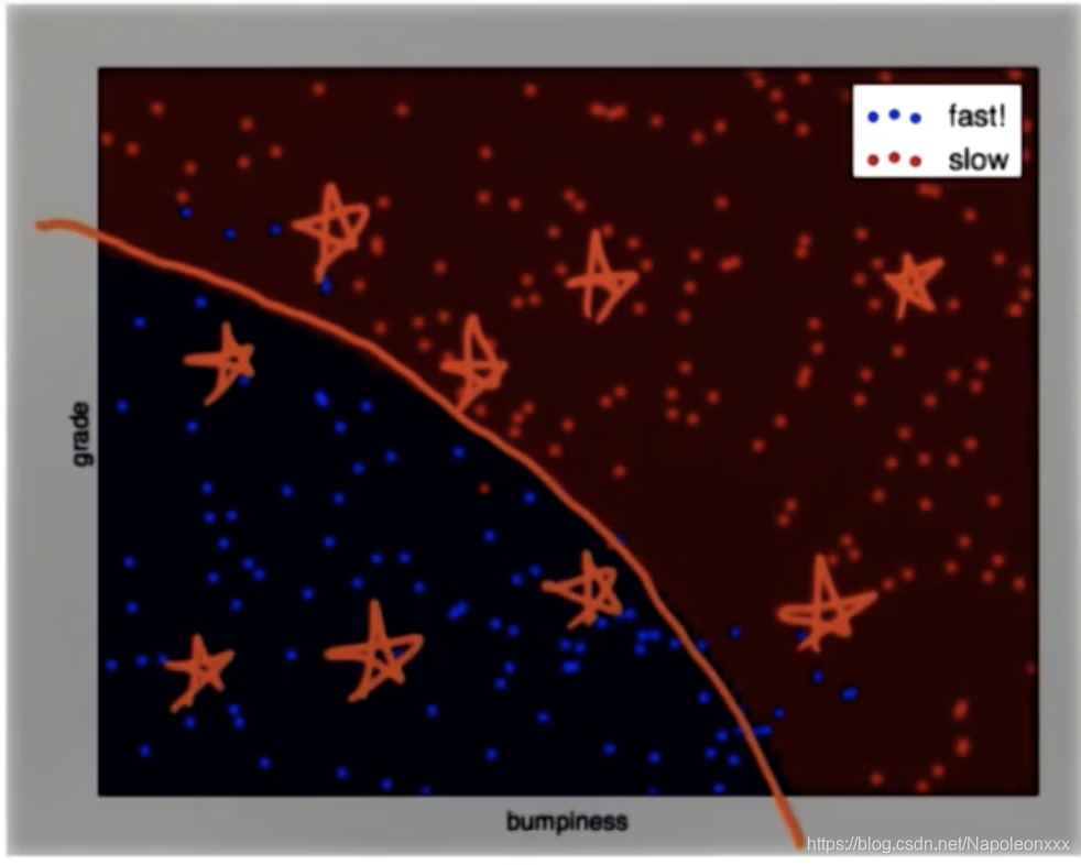
机器学习算法做的事情是定义了一个所谓的决策面(decision surface)。决策面通常位于两个不同类之间的某个位置上。当我们使用决策面，那么判断标记所属的分类就简单多了。可将决策面泛化为区分数据的不同类型，可以对之前从未出现的数据点进行分类。

当决策面是一条直线时，我们称它为线性决策面。

机器学习算法所做的是根据输入数据，将它们转化为一个决策面，简称为D.S.(Decision Surface)。对于后续所有情况可以帮你确定数据的分类。

朴素贝叶斯 (Naive Bayes)

是一个常用的寻找决策面的算法。属于监督分类算法

课程中的一个栗子是驾驶数据集，散点图上已经有750个点，我们的目的是绘制一条决策边界，帮助用户判断需要减速和可以快速行驶的地形。也就是将地形分为两类，在两个类之间画出决策边界。这样对于任意点，我们可以马上判断其属于那种地形以适应不同的速度。

贝叶斯初探

scikit-learn 是基于 Python 语言的机器学习工具。

• 简单高效的数据挖掘和数据分析工具
• 可供大家在各种环境中重复使用
• 建立在 NumPy ，SciPy 和 matplotlib 上
• 开源，可商业使用 - BSD许可证

在驾驶数据集的栗子中我们使用sklearn提供的 GaussianNB

from sklearn.naive_bayes import GaussianNB

第一步：创建一个模拟的驾驶数据集

#!/usr/bin/python
import random


def makeTerrainData(n_points=1000):
###############################################################################
### make the toy dataset
    random.seed(42)
    grade = [random.random() for ii in range(0,n_points)]
    bumpy = [random.random() for ii in range(0,n_points)]
    error = [random.random() for ii in range(0,n_points)]
    y = [round(grade[ii]*bumpy[ii]+0.3+0.1*error[ii]) for ii in range(0,n_points)]
    for ii in range(0, len(y)):
        if grade[ii]>0.8 or bumpy[ii]>0.8:
            y[ii] = 1.0

### split into train/test sets
    X = [[gg, ss] for gg, ss in zip(grade, bumpy)]
    split = int(0.75*n_points)
    X_train = X[0:split]
    X_test  = X[split:]
    y_train = y[0:split]
    y_test  = y[split:]

    grade_sig = [X_train[ii][0] for ii in range(0, len(X_train)) if y_train[ii]==0]
    bumpy_sig = [X_train[ii][1] for ii in range(0, len(X_train)) if y_train[ii]==0]
    grade_bkg = [X_train[ii][0] for ii in range(0, len(X_train)) if y_train[ii]==1]
    bumpy_bkg = [X_train[ii][1] for ii in range(0, len(X_train)) if y_train[ii]==1]

#    training_data = {"fast":{"grade":grade_sig, "bumpiness":bumpy_sig}
#            , "slow":{"grade":grade_bkg, "bumpiness":bumpy_bkg}}


    grade_sig = [X_test[ii][0] for ii in range(0, len(X_test)) if y_test[ii]==0]
    bumpy_sig = [X_test[ii][1] for ii in range(0, len(X_test)) if y_test[ii]==0]
    grade_bkg = [X_test[ii][0] for ii in range(0, len(X_test)) if y_test[ii]==1]
    bumpy_bkg = [X_test[ii][1] for ii in range(0, len(X_test)) if y_test[ii]==1]

    test_data = {"fast":{"grade":grade_sig, "bumpiness":bumpy_sig}
            , "slow":{"grade":grade_bkg, "bumpiness":bumpy_bkg}}

    return X_train, y_train, X_test, y_test
#    return training_data, test_data

第二步：用sklearn中的GaussianNB，创建一个分类器函数

def classify(features_train, labels_train):
    ### import the sklearn module for GaussianNB
    from sklearn.naive_bayes import GaussianNB
    ### create classifier
    clf = GaussianNB()
    ### fit the classifier on the training features and labels
    clf.fit(features_train, labels_train)
    ### return the fit classifier
    return clf

第三步：绘制散点图函数以及图像生成函数

#!/usr/bin/python

# from udacityplots import *
import warnings

warnings.filterwarnings("ignore")

import matplotlib

matplotlib.use('agg')

import matplotlib.pyplot as plt
import pylab as pl
import numpy as np


# import numpy as np
# import matplotlib.pyplot as plt
# plt.ioff()

def prettyPicture(clf, X_test, y_test):
    x_min = 0.0;
    x_max = 1.0
    y_min = 0.0;
    y_max = 1.0

    # Plot the decision boundary. For that, we will assign a color to each
    # point in the mesh [x_min, m_max]x[y_min, y_max].
    h = .01  # step size in the mesh
    xx, yy = np.meshgrid(np.arange(x_min, x_max, h), np.arange(y_min, y_max, h))
    Z = clf.predict(np.c_[xx.ravel(), yy.ravel()])

    # Put the result into a color plot
    Z = Z.reshape(xx.shape)
    plt.xlim(xx.min(), xx.max())
    plt.ylim(yy.min(), yy.max())

    plt.pcolormesh(xx, yy, Z, cmap=pl.cm.seismic)

    # Plot also the test points
    grade_sig = [X_test[ii][0] for ii in range(0, len(X_test)) if y_test[ii] == 0]
    bumpy_sig = [X_test[ii][1] for ii in range(0, len(X_test)) if y_test[ii] == 0]
    grade_bkg = [X_test[ii][0] for ii in range(0, len(X_test)) if y_test[ii] == 1]
    bumpy_bkg = [X_test[ii][1] for ii in range(0, len(X_test)) if y_test[ii] == 1]

    plt.scatter(grade_sig, bumpy_sig, color="b", label="fast")
    plt.scatter(grade_bkg, bumpy_bkg, color="r", label="slow")
    plt.legend()
    plt.xlabel("bumpiness")
    plt.ylabel("grade")

    plt.savefig("test.png")


import base64
import json
import subprocess


def output_image(name, format, bytes):
    image_start = "BEGIN_IMAGE_f9825uweof8jw9fj4r8"
    image_end = "END_IMAGE_0238jfw08fjsiufhw8frs"
    data = {}
    data['name'] = name
    data['format'] = format
    data['bytes'] = base64.encodestring(bytes)
    print image_start + json.dumps(data) + image_end

第四步：main函数输出结果

#!/usr/bin/python

""" Complete the code in ClassifyNB.py with the sklearn
    Naive Bayes classifier to classify the terrain data.

    The objective of this exercise is to recreate the decision
    boundary found in the lesson video, and make a plot that
    visually shows the decision boundary """

from prep_terrain_data import makeTerrainData
from class_vis import prettyPicture, output_image
from ClassifyNB import classify

import numpy as np
import pylab as pl

features_train, labels_train, features_test, labels_test = makeTerrainData()

### the training data (features_train, labels_train) have both "fast" and "slow" points mixed
### in together--separate them so we can give them different colors in the scatterplot,
### and visually identify them
grade_fast = [features_train[ii][0] for ii in range(0, len(features_train)) if labels_train[ii] == 0]
bumpy_fast = [features_train[ii][1] for ii in range(0, len(features_train)) if labels_train[ii] == 0]
grade_slow = [features_train[ii][0] for ii in range(0, len(features_train)) if labels_train[ii] == 1]
bumpy_slow = [features_train[ii][1] for ii in range(0, len(features_train)) if labels_train[ii] == 1]

# You will need to complete this function imported from the ClassifyNB script.
# Be sure to change to that code tab to complete this quiz.
clf = classify(features_train, labels_train)

### draw the decision boundary with the text points overlaid
prettyPicture(clf, features_test, labels_test)
output_image("test.png", "png", open("test.png", "rb").read())

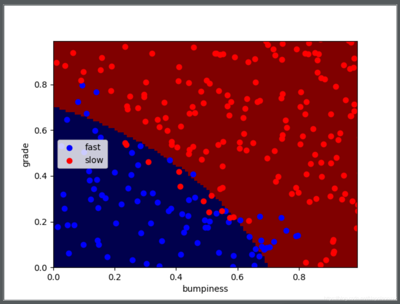
最后运行main函数，生成一张图片，结果如下：

贝叶斯规则–深入解析朴素贝叶斯

号称概率推理的圣杯—贝叶斯规则(Bayes Rule)。是一个广泛影响了人工智能和统计的全新方法体系。

以癌症发生率举例：
假如一种特定癌症发生率为人口的1%，对于这种癌症的检查：若得了这种癌症，检查结果90%可能是阳性的，这通常叫做测试的敏感性(sensitivity)。但有时你没有患癌症，检查结果还是呈阳性，所以我们假设，若你没有患上这种特定癌症，有90%的可能性是呈阴性，这通常叫做特异性(specitivity)。

第一个问题是：没有任何症状的情况下你进行了检查，检查结果呈阳性，你认为患上这种特定癌症的可能性是多少？

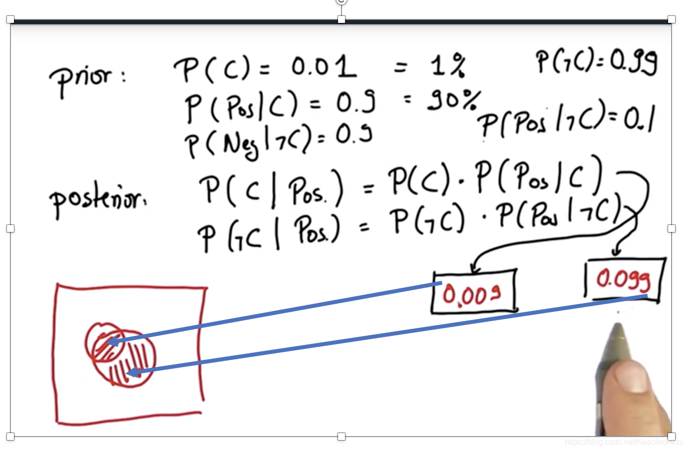
回答这个问题前，先直观上一张图：

下图的矩形代表所有人口，C的圆圈代表患癌的人。C+Pos代表患有癌症且检查为阳性的人(患癌人口中的90%)。然而这并不是全部真相，即使这个人没有患癌症，检查结果也可能呈阳性，即Pos ℸC，面积为整个矩形减去癌症圈C后的10%。显然这些圈以外的区域是没有患癌症且呈阴性的。

再来看第一个问题，该型癌症的先验概率为1%，敏感性和特异性为90%。计算结果大概为8%，即检查结果呈阳性，你认为患上这种特定癌症的可能性是8%。

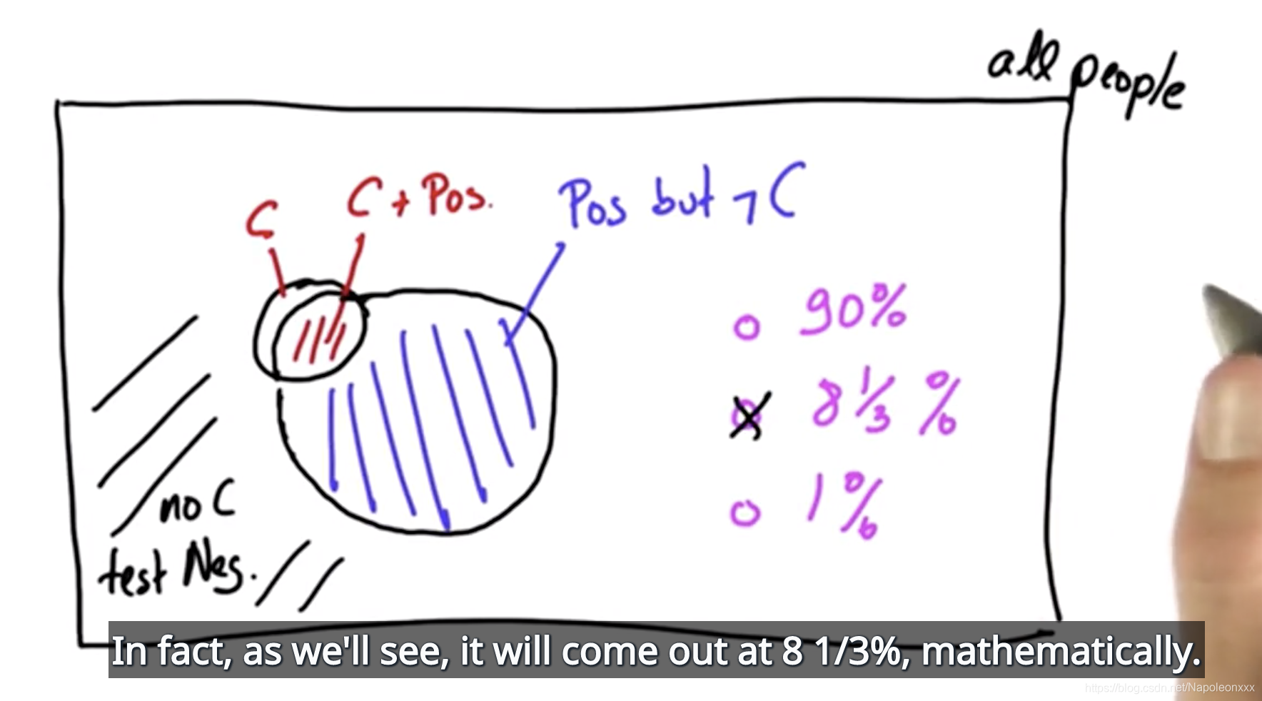
阳性区域即为C+Pos以及ℸC Pos之和。

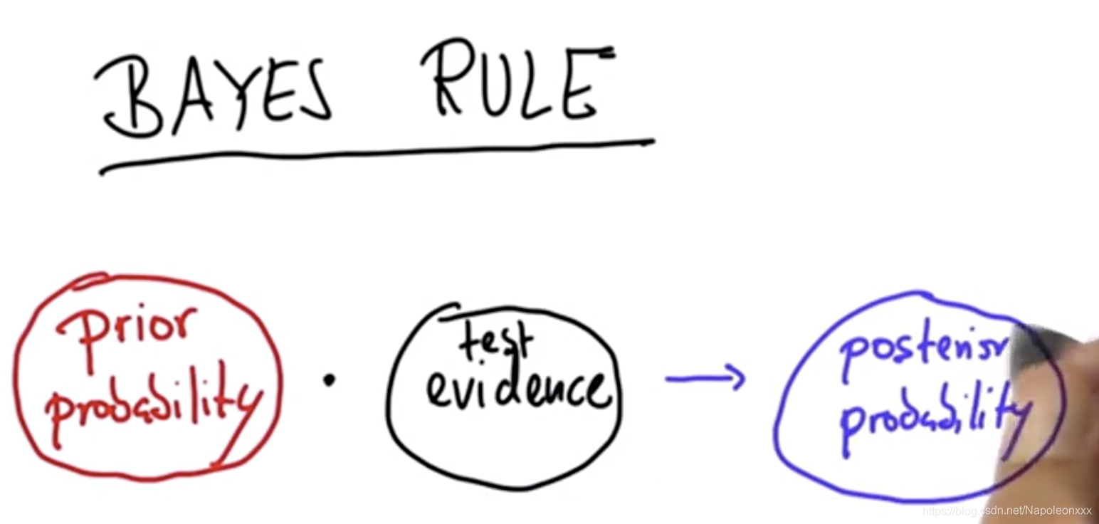
先验和后验

先验概率是检验之前所得到的概率。然后我们会从测试本身获得一些证据，这些会引导我们得出后验概率。

贝叶斯法则就是将测试中的某些证据加入先验概率中，以便获得后验概率

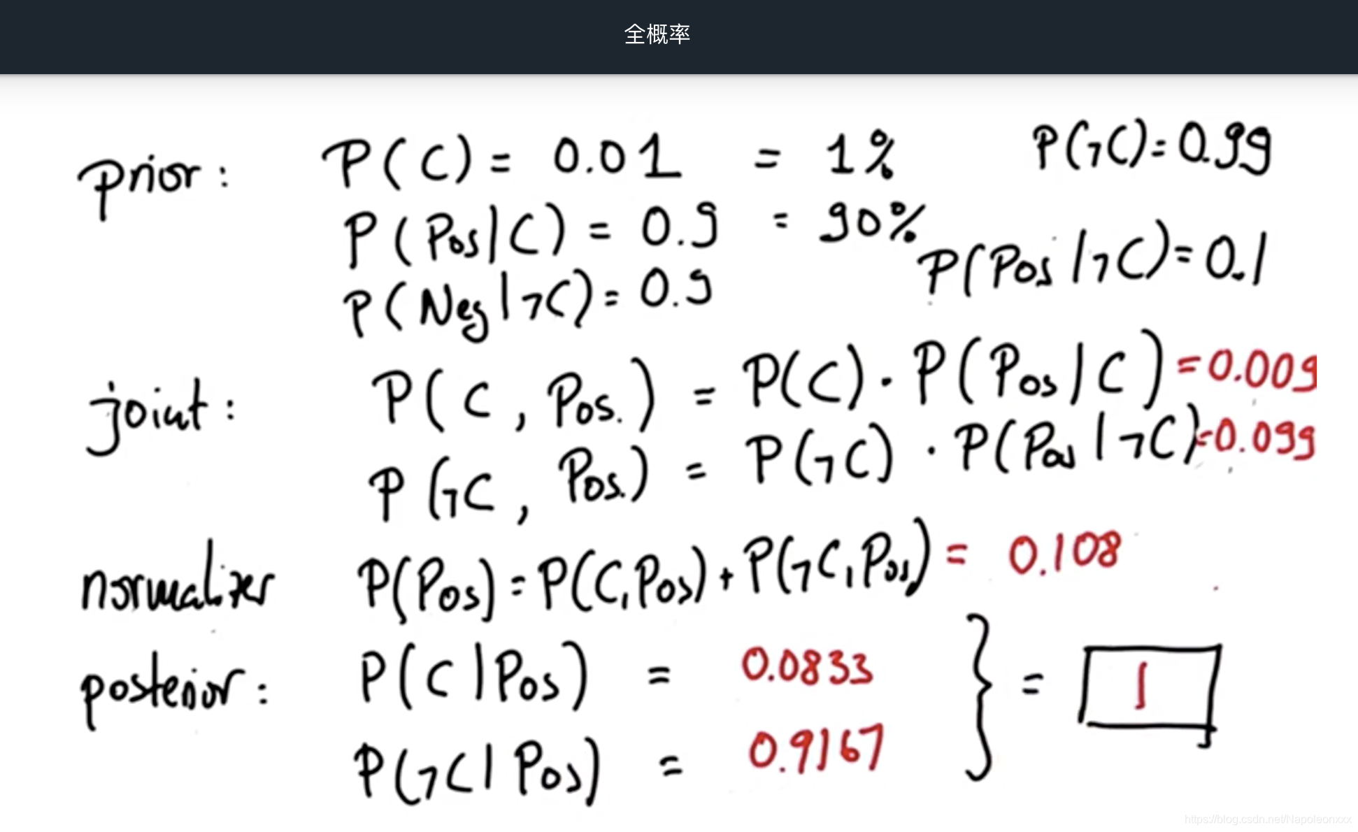
还以癌症测试为例：

勘误：上图中的后验概率应为联合概率:

P(C, Pos) = P( C ) • P(Pos|C)
P(ℸC, Pos) = P(ℸC)• P(Pos|ℸC)

我们发现P(ℸC|POS)和P(C|POS)的和并不是1，这是因为我们计算的是上图箭头指向框里面的绝对面积。

接下来是归一化即将我们的计算结果归一比例保持不变，但是确保它们相加之和为1.

贝叶斯规则图

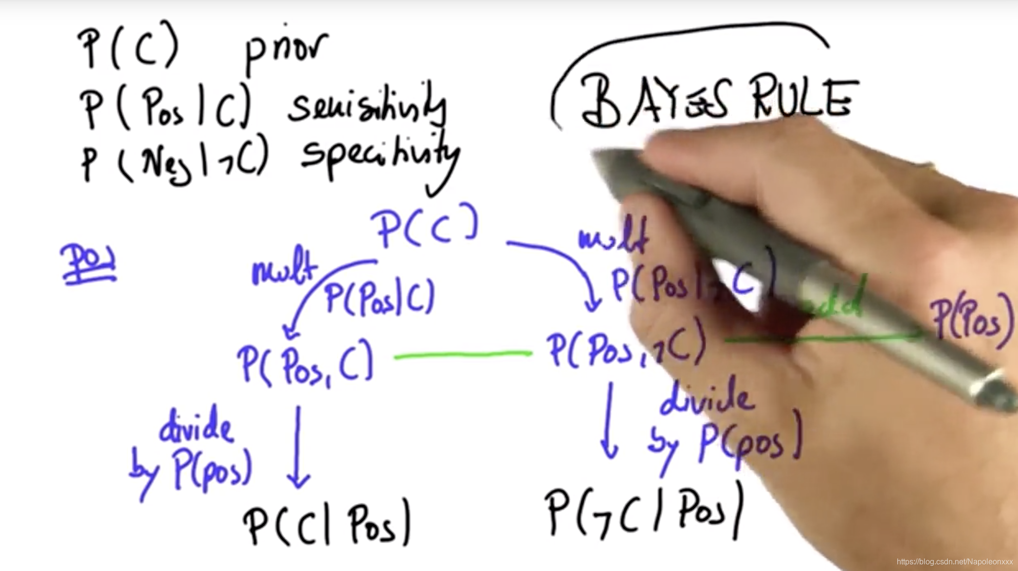
下图是对以上计算的一个总结

1） 栗子中首先有一个先验概率(prior)，以及敏感性(sensitivity)和特殊性(specificity)。

2）当我们得到一个阳性测试结果，我们要做的是获取先验结果，然后把此测试结果的概率分别乘以在C发生的情况(P(Pos|C))和C不发生的情况下(P(Pos|ℸC))获取相应检验结果的概率，即两个分支(患癌的分支和不患癌的分支)。完成此操作后我们将获得一个数字，该数字把患癌假设和测试结果结合了起来，包含了患癌假设P(Pos, C)和未患癌假设P(Pos, ℸC)，然后将这两个结果相加，它们的结果通常不会超过1，这刚好是测试结果在总样本中的概率。

3）最后通过归一化得到后验概率。

以上即为贝叶斯规则算法

用于分类的贝叶斯规则

假设有两个人Chris和Sara，二人都写了很多邮件，为简单起见，假设这些电子邮件仅包含了三个词语，爱，交易，生活。Chris和Sara的区别是他们使用这些词的频率不同。假设Chris喜欢谈论交易，他的词语中有80%涉及交易，他谈论爱和生活的概率为0.1。Sara更多的谈及爱，较少的谈及交易和生活，分别占0.2和0.3。

我们可以使用朴素贝叶斯方法基于随机邮件确定邮件的发送人。假设事先认定发送人是Chris或Sara的概率各为50%，即先验概率为50%。

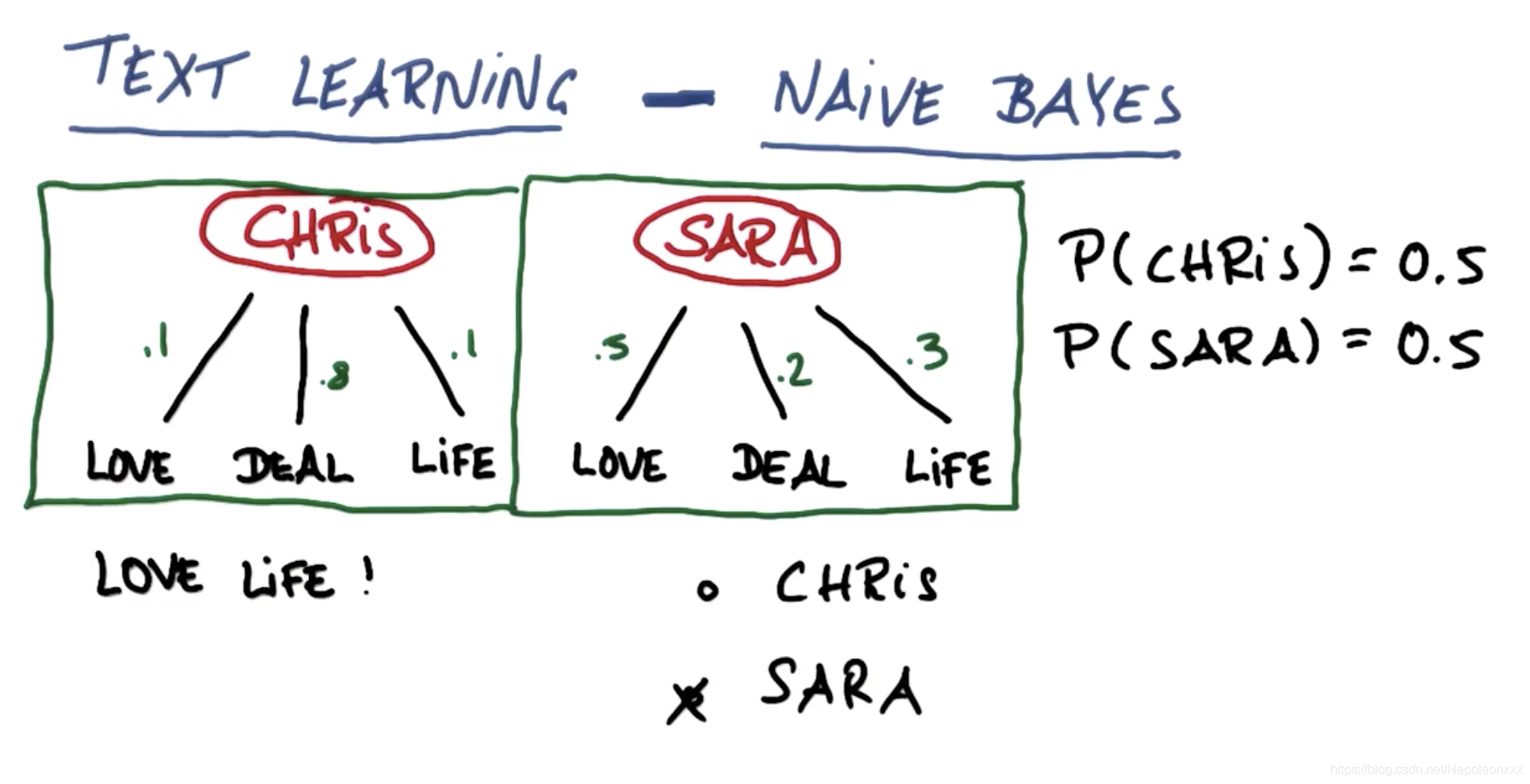
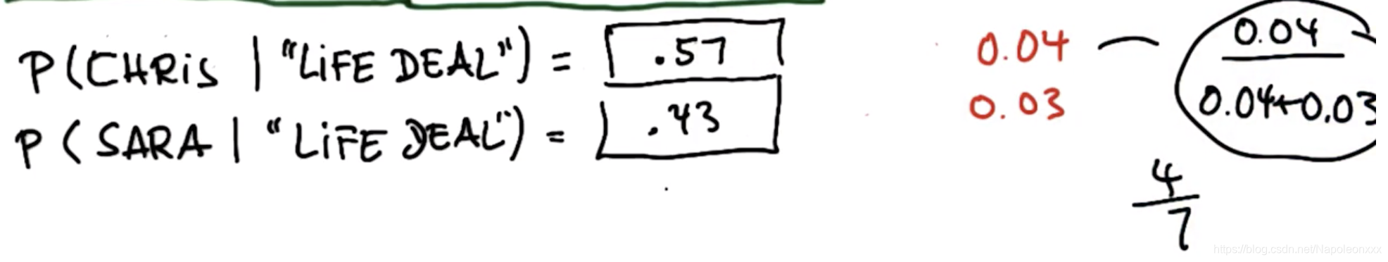
请看下题：一封邮件是关于生活和交易，那么谁的概率大一些：

第一步：得出联合概率

第二步： 归一化得出后验概率

为何朴素贝叶斯很朴素

以文本信息为例，我们之前的计算只是根据频率，却不关注信息里面词语的顺序，它被朴素的忽略了。所以这种方法并没有真正理解文本，它只能把词的频率当作一种分类方法，这就是为什么被称为朴素的原因。

朴素贝叶斯的优势和劣势

优势：算法非常容易执行，特征空间非常大，英语大概有2w到20w单词，该算法运行起来非常容易，效率非常高。

劣势：有时会失败，比如谷歌在早期使用这个算法时，搜索芝加哥公牛队，结果是芝加哥这座城市和公牛这种动物，所以由多个单词组成且意义明显不同的短语，朴素贝叶斯就不太适用了。所以我们需要训练集和测试集。用测试集来检验分类算法的表现，观察它如何运行。如果表现不尽如人意可能是算法不合适或者参数有误。