朴素贝叶斯(Naive Bayers)是一种基于概率统计的分类方法。它在条件独立的基础上,使用贝叶斯定理构建算法,在文本处理领域有广泛的应用。
一、基础知识理解
1、什么是条件概率?
条件概率是指事件A在另外一个事件B已经发生条件下的发生概率。
条件概率:表示为:P(A|B),读作“在B条件下A的概率”。若只有两个事件A,B,那么,
联合概率:表示两个事件共同发生的概率。A与B 的联合概率表示为 P(AB) 或者P (A,B ),或者P(A∩B)。
讲到条件概率不得不提到下面有名的红球蓝球实验
红球蓝球实验:在一个盒子中有5个红球和2个蓝球,连续拿2次,每次只能拿一颗球且不放回,求拿到2个蓝球的概率。

在计算概率之前,我们需要弄清楚,第1次拿球和第2次拿球是相关事件还是独立事件,很显然是相关事件,因为第1次拿球的结果,会影响第2次拿球的概率,他们是互相影响的,要连续拿到2个蓝球,那么第1次拿到的球就必须是蓝球。
如果把第1次拿到的球是蓝球的事件作为事件A,而第2次拿到的球是蓝球的事件作为事件B,那么连续拿到2个蓝球的概率,就是在事件A发生的条件下事件B也要发生的概率。
第1次拿到蓝球的概率P(A)=2/7,现在还剩下5个红球和1个蓝球,第2次拿到蓝球的概率为P(B|A)=1/6,那么连续拿到2个蓝球的概率P(AB)=P(A)*P(B|A)=(2/7)*(1/6)=1/21
求条件概率我们高中的时候就已经学过了,只不过那个时候学了用不到而已。
2、什么是贝叶斯定理?
贝叶斯定理其实就是一个条件概率公式,只不过跟上面的有点不一样,事件B发生的条件下事件A也要发生的概率。
贝叶斯定理的数学表达式:
借用维基百科上的一个案例来分析:
某警察小姐姐使用了一个假冒伪劣的醉驾呼气测试仪来检查司机是否醉驾?
先假设这种这个假冒伪劣产品(注意:不是我们公司研发的啊,不背锅)会把一个正常司机判为醉驾的概率是5%,而对醉驾的司机判为醉驾的概率是100%,然后警察小姐姐根据以前的统计得知,大概有0.1%的司机为醉驾。
此时,刚好过来一辆车,被小姐姐拦下检查,问该车司机是醉驾的概率有多大?
如果样本为1000个司机,1000*0.1%=1,那么只有一个司机是真正的醉驾,而其他999个司机是正常司机
被误判正常司机的个数:999*5%
真正醉驾司机的概率:P=1/(1+999*5%)=1.96%
我们再假设事件A为司机真正醉驾,事件B为仪器显示醉驾,那么案例要求的就是P(A|B),事件B发生的条件下事件A也要发生的概率。
先验概率(prior probability)是指根据以往经验和分析得到的概率。
那么事件A为司机真正醉驾的概率的概率P(A)=0.1%就是先验概率,根据以往经验和分析得到
那么醉驾司机被仪器显示为醉驾的概率P(B|A)=100%
那么仪器显示醉驾的概率P(B)=(0.1%+(1-0.1%)*5%)
而正常司机被误判的概率P()就是(1-0.1%)*5%
代入贝叶斯定理可得:(0.1%*100%)/[0.1%+(1-0.1%)*5%]=1.96%
3、朴素贝叶斯分类算法的原理?朴素是什么意思?
4、什么都是二项式分布?
5、多项式分布?
6、高斯分布?
7、高斯分布的概率密度函数在二维坐标轴上的形状是什么样的?
6、使用朴素贝叶斯分类法时,使用概率分布函数来计算概率,与从数据集里直接统计出概率相比,有什么优点?
二、朴素贝叶斯分类器通常有两种实现方式
1、一种基于伯努利模型实现
2、一种基于多项式模型实现
三、使用朴素贝叶斯进行文本分类
朴素贝叶斯的一般过程:
(1)收集数据:可以使用任何方法
(2)准备数据:需要数值型或者布尔型数据
(3)分析数据:有大量特征时,绘制特征作用不大,此时使用直方图效果更好
(4)训练算法:计算不同的独立特征的条件概率
(5)测试算法:计算错误率
(6)使用算法:一个常见的朴素贝叶斯应用是文档分类。可以在任意的分类场景中使用朴素贝叶斯分类器,不一定非要是文本
四、使用朴素贝叶斯进行文本分类(不调用scikit-learn机器学习库)
1、打开python编辑器(我用的JetBrains PyCharm 2017.2.4),创建一个bayes.py的python file
2、代码:
from numpy import *

# 创建了一些实验样本
def loadDataSet():
    postingList=[['my','dog','has','flea','problems','help','please'],['maybe','not','take','him','to','dog','park','stupid'],
                 ['my','dalmation','is','so','cute','i','love','him'],['stop','posting','stupid','worthless','garbage'],
                 ['mr','licks','ate','my','steak','how','to','stop','him'],['quit','buying','worthless','dog','food','stupid']]
    classVec=[0,1,0,1,0,1]  # 1代表侮辱性文字,0代表正常言论
    # 该函数返回的第一个变量是进行词条切分后的文档集合,这些文档来自斑犬爱好者留言板
    # 返回的第二个变量是一个类别标签的集合
    return postingList,classVec
# 创建一个包含在所有文档中出现的不重复词的列表
def createVocabList(dataSet): # postingList赋给dataSet
    vocabSet=set([])    # 创建一个空集
    for document in dataSet:
        vocabSet=vocabSet | set(document)   # 创建两个集合并集
    return list(vocabSet)
# 该函数的输入参数为词汇表及某个文档,输出的是文档向量,向量的每一元素为1或0,分别表示词汇表中的单词在输入文档中是否出现
def setOfWords2Vec(vocabList,inputSet):
    # 创建一个和词汇表等长的向量,并将其元素都设置为0
    returnVec=[0]*len(vocabList)
    # 遍历文档中的所有单词,如果出现了词汇表中的单词,则将输出的文档向量中的对应值设为1
    for word in inputSet:
        if word in vocabList:
            returnVec[vocabList.index(word)]=1
        else:
            print("the word:%s is not in my Vocabulary !") % word
    return returnVec

def trainNB0(trainMatrix,trainCategory) :
    numTrainDocs = len(trainMatrix)
    numWords = len(trainMatrix[0])
    pAbusive = sum(trainCategory) / float(numTrainDocs)
    p0Num = zeros(numWords);plNum = zeros(numWords)
    p0Denom = 0.0;plDenom = 0.0
    for i in range(numTrainDocs):
        if trainCategory[i] == 1:
            plNum += trainMatrix[i]
            plDenom += sum(trainMatrix[i])
        else :
            p0Num+=trainMatrix[i]
            p0Denom+=sum(trainMatrix[i])
    # 对每个元素做除法求概率
    p1Vect = plNum / plDenom
    p0Vect = p0Num / p0Denom
    # 返回两个类别概率向量和一个概率
    return p0Vect,p1Vect,pAbusive
3、创建一个test.py的python file用于测试输出结果
from numpy import *
import bayes

listOPosts,listClasses=bayes.loadDataSet()
myVocabList=bayes.createVocabList(listOPosts)
print(myVocabList)
print(bayes.setOfWords2Vec(myVocabList,listOPosts[0]))  # 排序
print(bayes.setOfWords2Vec(myVocabList,listOPosts[1]))  # 排序
print(bayes.setOfWords2Vec(myVocabList,listOPosts[2]))  # 排序
print(bayes.setOfWords2Vec(myVocabList,listOPosts[3]))  # 排序

listOPosts,listClasses=bayes.loadDataSet()
myVocabList = bayes.createVocabList(listOPosts)
trainMat=[]
for postinDoc in listOPosts:
    trainMat.append(bayes.setOfWords2Vec(myVocabList,postinDoc))

p0V,plV,pAb=bayes.trainNB0(trainMat, listClasses)
print(pAb)  # 变量的内部值
print(p0V)  # 任意文档属于侮辱性文档的概率
print(plV)  # 任意文档属于非侮辱性文档的概率
4、输出结果:
['garbage', 'food', 'park', 'problems', 'cute', 'i', 'how', 'stop', 'love', 'steak', 'dalmation', 'mr', 'help', 'maybe', 'not', 'my', 'has', 'him', 'flea', 'take', 'dog', 'stupid', 'quit', 'posting', 'please', 'buying', 'to', 'licks', 'worthless', 'ate', 'so', 'is']
[0, 0, 0, 1, 0, 0, 0, 0, 0, 0, 0, 0, 1, 0, 0, 1, 1, 0, 1, 0, 1, 0, 0, 0, 1, 0, 0, 0, 0, 0, 0, 0]
这个输出结果中的‘1’表示:'problems'、'help'、'my'、'has'、'flea'、'dog'、'please'在创建的词汇样本的第一个列表中出现了,而‘0’表示未出现
[0, 0, 1, 0, 0, 0, 0, 0, 0, 0, 0, 0, 0, 1, 1, 0, 0, 1, 0, 1, 1, 1, 0, 0, 0, 0, 1, 0, 0, 0, 0, 0][0, 0, 0, 0, 1, 1, 0, 0, 1, 0, 1, 0, 0, 0, 0, 1, 0, 1, 0, 0, 0, 0, 0, 0, 0, 0, 0, 0, 0, 0, 1, 1]
[1, 0, 0, 0, 0, 0, 0, 1, 0, 0, 0, 0, 0, 0, 0, 0, 0, 0, 0, 0, 0, 1, 0, 1, 0, 0, 0, 0, 1, 0, 0, 0]
0.5
[ 0. 0. 0. 0.04166667 0.04166667 0.04166667
0.04166667 0.04166667 0.04166667 0.04166667 0.04166667 0.04166667
0.04166667 0. 0. 0.125 0.04166667 0.08333333
0.04166667 0. 0.04166667 0. 0. 0.
0.04166667 0. 0.04166667 0.04166667 0. 0.04166667
0.04166667 0.04166667]
[ 0.05263158 0.05263158 0.05263158 0. 0. 0. 0.
0.05263158 0. 0. 0. 0. 0.
0.05263158 0.05263158 0. 0. 0.05263158 0.
0.05263158 0.10526316 0.15789474 0.05263158 0.05263158 0.
0.05263158 0.05263158 0. 0.10526316 0. 0. 0. ]
五、使用朴素贝叶斯进行文本分类(调用scikit-learn机器学习库)
准备部分:【加载需要使用的类库和模块】
from time import time
from sklearn.datasets import load_files
from sklearn.feature_extraction.text import TfidfVectorizer
from sklearn.naive_bayes import MultinomialNB
from sklearn.metrics import classification_report
from sklearn.metrics import confusion_matrix
# %matplotlib inline:IPython的魔法函数
import matplotlib.pyplot as plt
第一部分:【把训练用的语料库读入内存】
# 第一部分:把训练用的语料库读入内存
print("loading train dataset ...")
t = time()
news_train = load_files('E:/Python_Project/《机器学习实战》/datasets/mlcomp/dataset-379-20news-18828/379/train')
# news_train.data是一个数组,里面包含了所有文档的文本信息;news_train.target_names类别名称
print("summary: {0} documents in {1} categories.".format(len(news_train.data), len(news_train.target_names)))
# news_train.target也是一个数组,包含了所有文档的所属类别,news_train.target[0]第一个类别
print('categories 1 name is : {0}'.format(news_train.target_names[news_train.target[0]]))
print("done in {0} seconds".format(time() - t))
输出结果:
loading train dataset ...
summary: 13180 documents in 20 categories.
categories 1 name is : talk.politics.misc
done in 1.0556299686431885 seconds
第二部分:【把文档全部转换为由TF-IDF表达的权重信息构成的向量】
# 第二部分:把文档全部转换为由TF-IDF表达的权重信息构成的向量
print("vectorizing train dataset ...")  # vectorizing train dataset:向量化训练数据
t = time()
# TfidfVectorizer类用来所有的文档转换为矩阵
vectorizer = TfidfVectorizer(encoding='latin-1')
# fit_transform方法是fit()和transform()的结合,fit()完成语料库分析、提取词典等操作,transform()会对每篇文档转换为向量,构成一个矩阵,保存在X_train中
X_train = vectorizer.fit_transform((d for d in news_train.data))
print("n_samples: %d, n_features: %d" % X_train.shape)
print("number of non-zero features in sample [{0}]: {1}".format(news_train.filenames[0], X_train[0].getnnz()))  # 不重复单词数量
print("done in {0} seconds".format(time() - t))
输出结果:
vectorizing train dataset ...
n_samples: 13180, n_features: 130274
number of non-zero features in sample [E:/Python_Project/《机器学习实战》/datasets/mlcomp/dataset-379-20news-18828/379/train\talk.politics.misc\17860-178992]: 108
done in 4.355855941772461 seconds
第三部分:【模型训练】
print("traning models ...".format(time() - t))
t = time()
y_train = news_train.target
# alpha值表示平滑参数,其值越小,越容易造成过拟合,值太大,容易造成欠拟合
clf = MultinomialNB(alpha=0.0001)
clf.fit(X_train, y_train)
# train_score:训练分数
train_score = clf.score(X_train, y_train)
print("train score: {0}".format(train_score))
print("done in {0} seconds".format(time() - t))
输出结果:
traning models ...
train score: 0.9978755690440061
done in 0.28122925758361816 seconds
第四部分:【加载测试数据集】
print("loading test dataset ...")
t = time()
news_test = load_files('E:/Python_Project/《机器学习实战》/datasets/mlcomp/dataset-379-20news-18828/379/test')
print("summary: {0} documents in {1} categories.".format(len(news_test.data), len(news_test.target_names)))
print("done in {0} seconds".format(time() - t))
输出结果:
loading test dataset ...
summary: 5648 documents in 20 categories.
done in 0.45315122604370117 seconds
第五部分:【把测试数据集文档向量化】
print("vectorizing test dataset ...")
t = time()
X_test = vectorizer.transform((d for d in news_test.data))
y_test = news_test.target
print("n_samples: %d, n_features: %d" % X_test.shape)
print("number of non-zero features in sample [{0}]: {1}".format(news_test.filenames[0], X_test[0].getnnz()))
print("done in %fs" % (time() - t))
输出结果:
vectorizing test dataset ...
n_samples: 5648, n_features: 130274
number of non-zero features in sample [E:/Python_Project/《机器学习实战》/datasets/mlcomp/dataset-379-20news-18828/379/test\rec.autos\7429-103268]: 61
done in 1.655229s
第六部分:【预测某一片文档的所属类别】
pred = clf.predict(X_test[0])
print("predict: {0} is in category {1}".format(news_test.filenames[0], news_test.target_names[pred[0]]))
print("actually: {0} is in category {1}".format(news_test.filenames[0], news_test.target_names[news_test.target[0]]))
输出结果:
predict: E:/Python_Project/《机器学习实战》/datasets/mlcomp/dataset-379-20news-18828/379/test\rec.autos\7429-103268 is in category rec.autos
actually: E:/Python_Project/《机器学习实战》/datasets/mlcomp/dataset-379-20news-18828/379/test\rec.autos\7429-103268 is in category rec.autos
第七部分:【对测试数据集进行预测】
print("predicting test dataset ...")
t = time()
pred = clf.predict(X_test)
print("done in %fs" % (time() - t))
输出结果:
predicting test dataset ...
done in 0.031272s
第八部分:【查看每个类别的预测准确性】
print("classification report on test set for classifier:")
print(clf)
print(classification_report(y_test, pred,target_names=news_test.target_names))
输出结果:
classification report on test set for classifier:
MultinomialNB(alpha=0.0001, class_prior=None, fit_prior=True)
                          precision    recall  f1-score   support

             alt.atheism       0.90      0.91      0.91       245
           comp.graphics       0.80      0.90      0.85       298
 comp.os.ms-windows.misc       0.82      0.79      0.80       292
comp.sys.ibm.pc.hardware       0.81      0.80      0.81       301
   comp.sys.mac.hardware       0.90      0.91      0.91       256
          comp.windows.x       0.88      0.88      0.88       297
            misc.forsale       0.87      0.81      0.84       290
               rec.autos       0.92      0.93      0.92       324
         rec.motorcycles       0.96      0.96      0.96       294
      rec.sport.baseball       0.97      0.94      0.96       315
        rec.sport.hockey       0.96      0.99      0.98       302
               sci.crypt       0.95      0.96      0.95       297
         sci.electronics       0.91      0.85      0.88       313
                 sci.med       0.96      0.96      0.96       277
               sci.space       0.94      0.97      0.96       305
  soc.religion.christian       0.93      0.96      0.94       293
      talk.politics.guns       0.91      0.96      0.93       246
   talk.politics.mideast       0.96      0.98      0.97       296
      talk.politics.misc       0.90      0.90      0.90       236
      talk.religion.misc       0.89      0.78      0.83       171

             avg / total       0.91      0.91      0.91      5648
第九部分:【通过confusion_matrix()函数生成混淆矩阵,观察每种类别被错误分类的情况】
cm = confusion_matrix(y_test, pred)
print("confusion matrix:")
print(cm)
输出结果:
confusion matrix:
[[224   0   0   0   0   0   0   0   0   0   0   0   0   0   2   5   0   0    1  13]
 [  1 267   5   5   2   8   1   1   0   0   0   2   3   2   1   0   0   0    0   0]
 [  1  13 230  24   4  10   5   0   0   0   0   1   2   1   0   0   0   0    1   0]
 [  0   9  21 242   7   2  10   1   0   0   1   1   7   0   0   0   0   0    0   0]
 [  0   1   5   5 233   2   2   2   1   0   0   3   1   0   1   0   0   0    0   0]
 [  0  20   6   3   1 260   0   0   0   2   0   1   0   0   2   0   2   0    0   0]
 [  0   2   5  12   3   1 235  10   2   3   1   0   7   0   2   0   2   1    4   0]
 [  0   1   0   0   1   0   8 300   4   1   0   0   1   2   3   0   2   0    1   0]
 [  0   1   0   0   0   2   2   3 283   0   0   0   1   0   0   0   0   0    1   1]
 [  0   1   1   0   1   2   1   2   0 297   8   1   0   1   0   0   0   0    0   0]
 [  0   0   0   0   0   0   0   0   2   2 298   0   0   0   0   0   0   0    0   0]
 [  0   1   2   0   0   1   1   0   0   0   0 284   2   1   0   0   2   1    2   0]
 [  0  11   3   5   4   2   4   5   1   1   0   4 266   1   4   0   1   0    1   0]
 [  1   1   0   1   0   2   1   0   0   0   0   0   1 266   2   1   0   0    1   0]
 [  0   3   0   0   1   1   0   0   0   0   0   1   0   1 296   0   1   0    1   0]
 [  3   1   0   1   0   0   0   0   0   0   1   0   0   2   1 280   0   1    1   2]
 [  1   0   2   0   0   0   0   0   1   0   0   0   0   0   0   0 236   1    4   1]
 [  1   0   0   0   0   1   0   0   0   0   0   0   0   0   0   3   0 290    1   0]
 [  2   1   0   0   1   1   0   1   0   0   0   0   0   0   0   1  10   7    212 0]
 [ 16   0   0   0   0   0   0   0   0   0   0   0   0   0   0  12   4   1    4   134]]
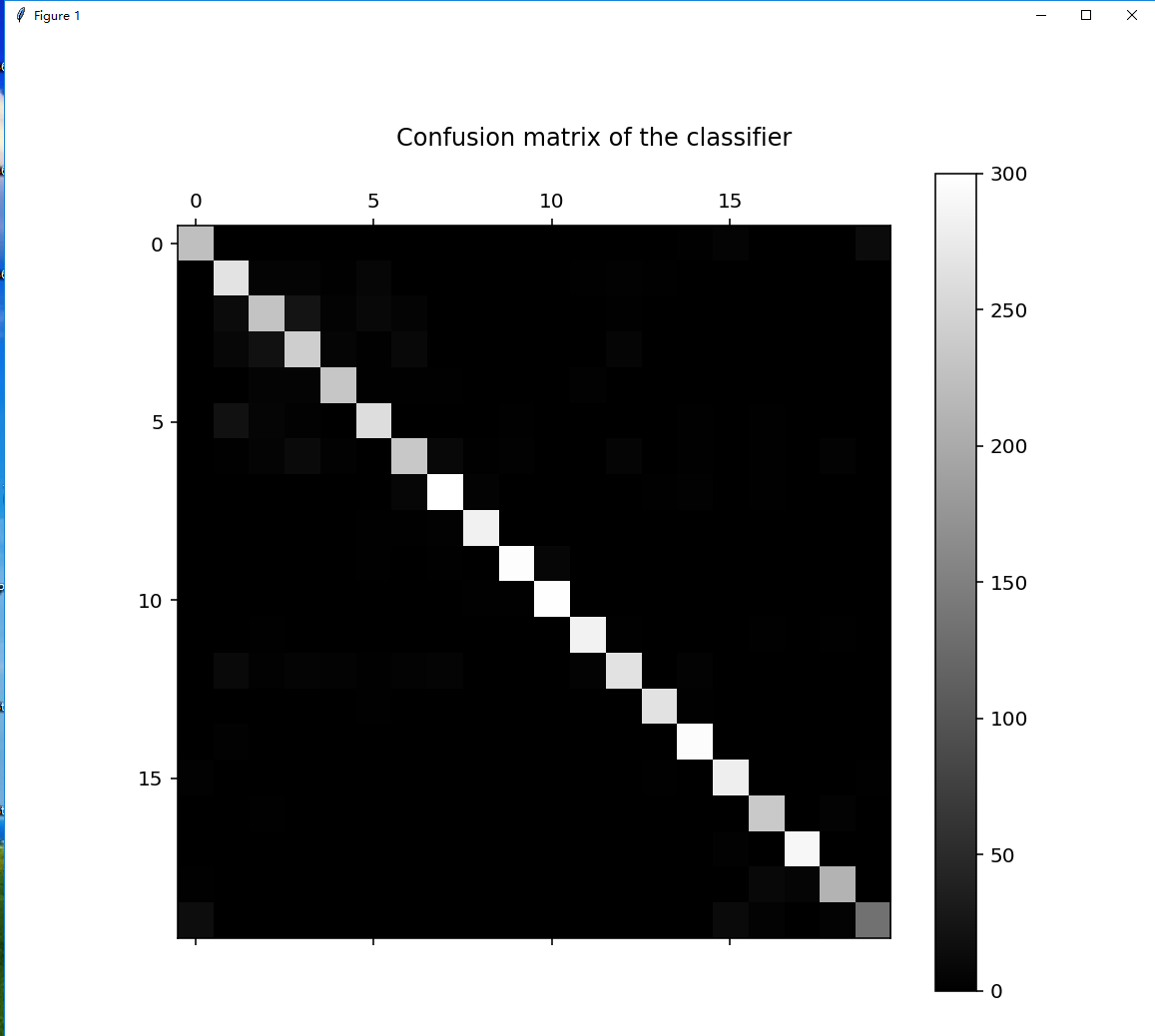
第十部分:【将混淆矩阵进行可视化处理】
plt.figure(figsize=(8, 8), dpi=144)
plt.title('Confusion matrix of the classifier')
ax = plt.gca()
ax.spines['right'].set_color('none')
ax.spines['top'].set_color('none')
ax.spines['bottom'].set_color('none')
ax.spines['left'].set_color('none')
ax.xaxis.set_ticks_position('none')
ax.yaxis.set_ticks_position('none')
ax.set_xticklabels([])
ax.set_yticklabels([])
plt.matshow(cm, fignum=1, cmap='gray')
plt.colorbar();
plt.show()
输出结果:
【全部代码】
from time import time
from sklearn.datasets import load_files
from sklearn.feature_extraction.text import TfidfVectorizer
from sklearn.naive_bayes import MultinomialNB
from sklearn.metrics import classification_report
from sklearn.metrics import confusion_matrix
# %matplotlib inline:IPython的魔法函数
import matplotlib.pyplot as plt


# 第一部分:把训练用的语料库读入内存
print("loading train dataset ...")
t = time()
news_train = load_files('E:/Python_Project/《机器学习实战》/datasets/mlcomp/dataset-379-20news-18828/379/train')
# news_train.data是一个数组,里面包含了所有文档的文本信息;news_train.target_names类别名称
print("summary: {0} documents in {1} categories.".format(len(news_train.data), len(news_train.target_names)))
# news_train.target也是一个数组,包含了所有文档的所属类别,news_train.target[0]第一个类别
print('categories 1 name is : {0}'.format(news_train.target_names[news_train.target[0]]))
print("done in {0} seconds".format(time() - t))

# 第二部分:把文档全部转换为由TF-IDF表达的权重信息构成的向量
print("vectorizing train dataset ...")  # vectorizing train dataset:向量化训练数据
t = time()
# TfidfVectorizer类用来所有的文档转换为矩阵
vectorizer = TfidfVectorizer(encoding='latin-1')
# fit_transform方法是fit()和transform()的结合,fit()完成语料库分析、提取词典等操作,transform()会对每篇文档转换为向量,构成一个矩阵,保存在X_train中
X_train = vectorizer.fit_transform((d for d in news_train.data))
print("n_samples: %d, n_features: %d" % X_train.shape)
print("number of non-zero features in sample [{0}]: {1}".format(news_train.filenames[0], X_train[0].getnnz()))  # 不重复单词数量
print("done in {0} seconds".format(time() - t))

# 第三部分:模型训练
print("traning models ...".format(time() - t))
t = time()
y_train = news_train.target
# alpha值表示平滑参数,其值越小,越容易造成过拟合,值太大,容易造成欠拟合
clf = MultinomialNB(alpha=0.0001)
clf.fit(X_train, y_train)
# train_score:训练分数
train_score = clf.score(X_train, y_train)
print("train score: {0}".format(train_score))
print("done in {0} seconds".format(time() - t))

# 第四部分:加载测试数据集
print("loading test dataset ...")
t = time()
news_test = load_files('E:/Python_Project/《机器学习实战》/datasets/mlcomp/dataset-379-20news-18828/379/test')
print("summary: {0} documents in {1} categories.".format(len(news_test.data), len(news_test.target_names)))
print("done in {0} seconds".format(time() - t))

# 第五部分:把测试数据集文档向量化
print("vectorizing test dataset ...")
t = time()
X_test = vectorizer.transform((d for d in news_test.data))
y_test = news_test.target
print("n_samples: %d, n_features: %d" % X_test.shape)
print("number of non-zero features in sample [{0}]: {1}".format(news_test.filenames[0], X_test[0].getnnz()))
print("done in %fs" % (time() - t))

# 第六部分:预测某一片文档的所属类别
pred = clf.predict(X_test[0])
print("predict: {0} is in category {1}".format(news_test.filenames[0], news_test.target_names[pred[0]]))
print("actually: {0} is in category {1}".format(news_test.filenames[0], news_test.target_names[news_test.target[0]]))

# 第七部分:对测试数据集进行预测
print("predicting test dataset ...")
t = time()
pred = clf.predict(X_test)
print("done in %fs" % (time() - t))

# 第八部分:查看每个类别的预测准确性
print("classification report on test set for classifier:")
print(clf)
print(classification_report(y_test, pred,target_names=news_test.target_names))

# 第九部分:通过confusion_matrix()函数生成混淆矩阵,观察每种类别被错误分类的情况
cm = confusion_matrix(y_test, pred)
print("confusion matrix:")
print(cm)

# 第十部分:将混淆矩阵进行可视化处理
plt.figure(figsize=(8, 8), dpi=144)
plt.title('Confusion matrix of the classifier')
ax = plt.gca()
ax.spines['right'].set_color('none')
ax.spines['top'].set_color('none')
ax.spines['bottom'].set_color('none')
ax.spines['left'].set_color('none')
ax.xaxis.set_ticks_position('none')
ax.yaxis.set_ticks_position('none')
ax.set_xticklabels([])
ax.set_yticklabels([])
plt.matshow(cm, fignum=1, cmap='gray')
plt.colorbar();
plt.show()
参考书籍:
1、《scikit-learn机器学习常用算法原理及编程实践》黄永昌编著
2、《机器学习实战》Peter Harrington编著