引言
上一章节,我们学习了CNN模型的发展历史和应用领域,同时细致的剖析了模型的结构和原理,也简单的学习了在TensorFlow内有关CNN的api。最后在MNIST和CIFAR10数据集上验证了CNN模型强大的特征提取能力。
本章节将学习经典的CNN模型,这几个CNN模型都曾在ImageNet大赛上大放光彩,也代表着这几年CNN模型的发展路线。
本节重点放在AlexNet和VGGNet上,下面表格是两个网络的简单比较:
| 特点 | AlexNet | VGGNet |
|---|---|---|
| 论文贡献 | 介绍完整CNN架构模型(近些年的许多CNN模型都是依据此模型变种来的)和多种训练技巧 CNN模型复兴的开山之作 使用GPU加速训练,让CNN模型训练得以实现 |
讨论了在小卷积核下,模型性能随着堆叠层数加深的变化 同时探讨multi-crop和dense evaluation对模型性能的影响 |
| 网络结构 | 1.AlexNet的网络架构成为了大型CNN模型的经典架构 2.成功的使用了ReLU激活函数 3.成功的应用了(重叠)最大池化层 |
1.多个小卷积核层堆叠(模型的迁移性能较好) 2.使用1*1卷积核增强模型的判别能力 |
| 训练Tricks | 1.数据增强,包括对训练数据做取RGB均值,随机截取固定尺寸,做水平翻转扩大训练集; 2.使用dropout技术增强模型的鲁棒性和泛化能力 3.测试时,对测试图片做数据增强,同时在softmax层去均值再输出 4.带动量的权值衰减 5.学习率在验证集上的错误率不提高时下降10倍 |
训练简单模型A,使用模型A的权值初始化复杂模型B(迁移学习) 数据增强,对训练数据去RGB均值,做水平翻转扩大训练集; 使用dropout技术 测试时,对测试图片做数据增强,在softmax层 带动量的权值衰减 学习率在验证集上的错误率不提高时下降10倍 |
| 其他观点 | LRN层有助于增强模型泛化能力 | LRN效果甚微,反倒的计算量增加不少 |
AlexNet
AlexNet 简介
2012年,Hinton的学生Alex提出了CNN模型AlexNet,AlexNet可以算是LeNet的一种更深更宽的版本。同年AlexNet以显著优势获得了IamgeNet的冠军,top-5错误率降低到了16.4%,相比于第二名26.2%的错误路有了巨大的提升,而AlexNet模型的参数量还不到第二名模型的二分之一。AlexNet可以说是神经网络在低谷期后第一次发威,确立了深度学习在计算机视觉领域的统治地位,同时也推动了深度学习在语音识别、自然语言处理、强化学习等领域的拓展。
AlexNet的特点
- 针对网络架构:
- 成功的使用ReLU作为激活函数,并验证其效果在较深的网络要优于Sigmoid.
- 使用LRN层,对局部神经元的活动创建竞争机制,使得其中响应比较大的值变的相对更大,并抑制其他反馈较小的神经元,增强了模型的泛化能力。
- 使用重叠的最大池化,论文中提出让步长比池化核的尺寸小,这样池化层的输出之间会有重叠和覆盖,提升了特征的丰富性。
- 针对过拟合现象:
- 数据增强,对原始图像随机的截取输入图片尺寸大小(以及对图像作水平翻转操作),使用数据增强后大大减轻过拟合,提升模型的泛化能力。同时,论文中会对原始数据图片的RGB做PCA分析,并对主成分做一个标准差为0.1的高斯扰动。
- 使用Dropout随机忽略一部分神经元,避免模型过拟合。
- 针对训练速度:
- 使用GPU计算,加快计算速度
AlexNet论文分析
引言
| 原文 | description |
|---|---|
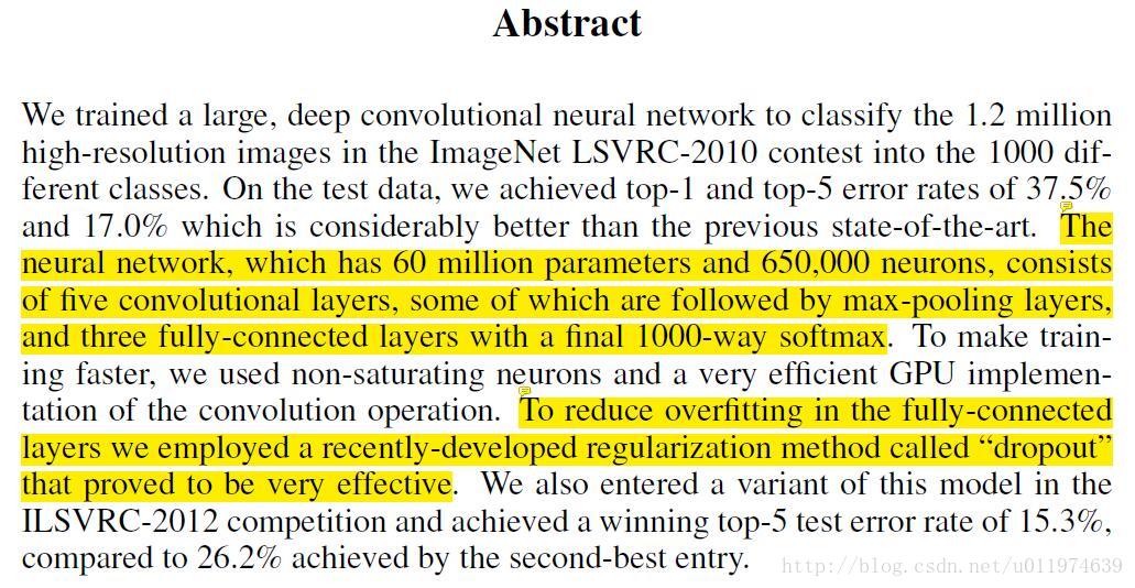
| The neural network, which has 60 million parameters and 650,000 neurons, consists of five convolutional layers, some of which are followed by max-pooling layers,and three fully-connected layers with a final 1000-way softmax. |
介绍了AlexNet网络结构: 五个卷积层(若干卷积层包含最大池化层)三个全连接层(最后一层为1000分类的softmax) 超过六千万参数和六十五万神经元 |
| To reduce overfitting in the fully-connected layers we employed a recently-developed regularization method called “dropout” that proved to be very effective. | 减少全连接层的过拟合情况: 使用dropout方法防治overfitting (后续有详解) |
1. 介绍
| 原文 | description |
|---|---|
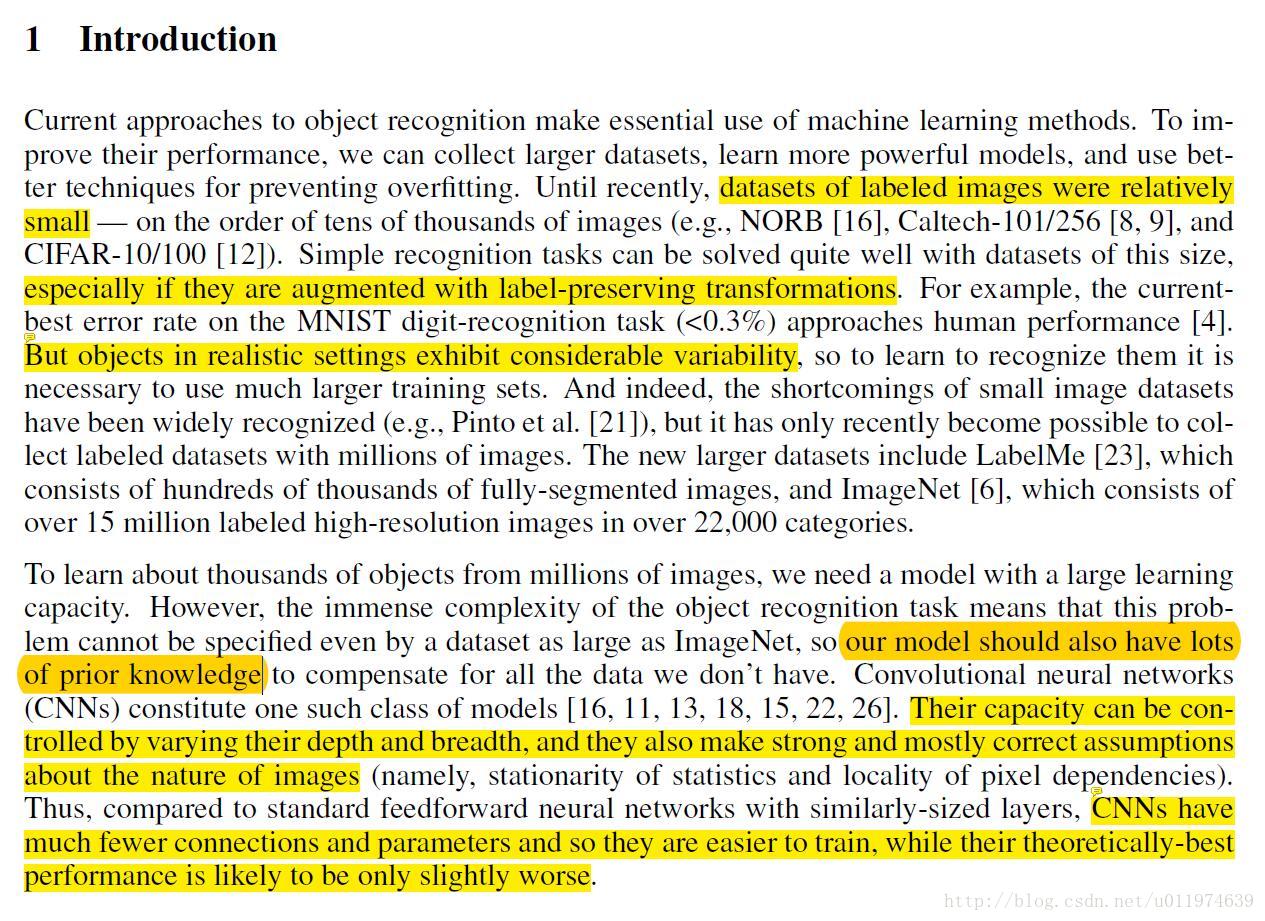
| datasets of labeled images were relatively small… especially if they are augmented with label-preserving transformations… But objects in realistic settings exhibit considerable variability… |
指出传统数据集和模型存在的问题: 数据集较小时,通过数据增强等技术,模型可在简单的识别任务上表现很好 但是在现实复杂环境识别任务上表现的不尽人意 进而引出了ImageNet数据集 |
| so our model should also have lots of prior knowledge Their capacity can be controlled by varying their depth and breadth and they also make strong and mostly correct assumptions about the nature of images CNNs have much fewer connections and parameters and so they are easier to train, while their theoretically-best performance is likely to be only slightly worse. |
点出为什么用CNN模型,CNN模型的优点? 我们的模型需要足够的先验知识 CNN的性能可以通过扩展宽度和深度来控制 CNN的参数相对来说较少,从而可训练 CNN的表现可观 |
| 原文 | description |
|---|---|
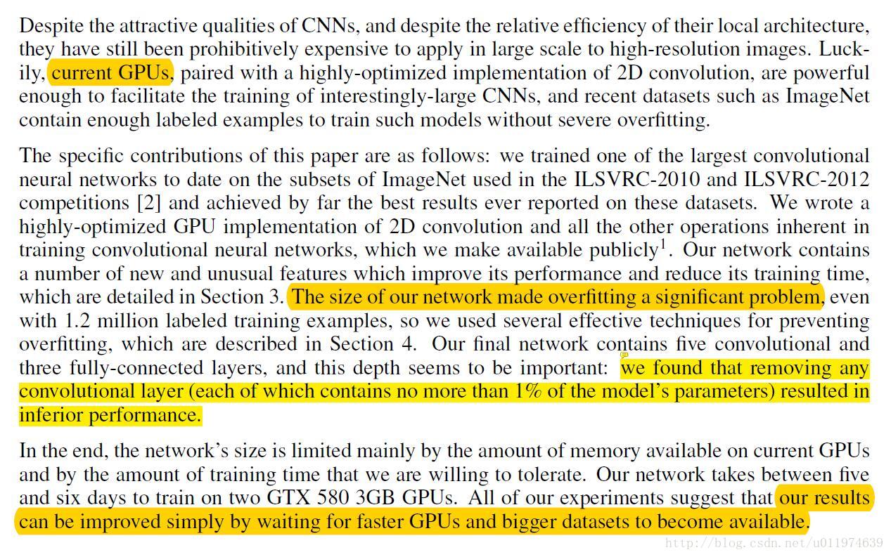
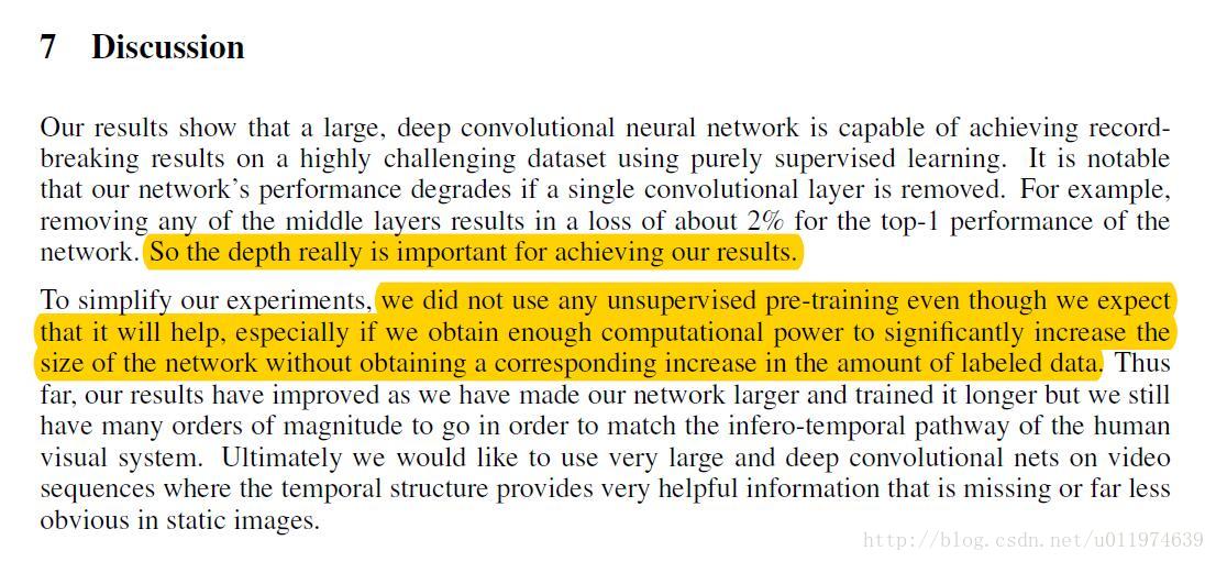
| current GPUs The size of our network made overfitting a significant problem we found that removing any convolutional layer resulted in inferior performance. our results can be improved simply by waiting for faster GPUs and bigger datasets to become available. |
CNN模型优缺点: 因为GPU,现在可以实现CNN模型的训练 这样多参数的模型,过拟合现象依旧是一个大问题 模型的深度看起来看重要,移除任何一个卷积层,模型的性能都会大大降低 提升模型性能简单的方法是使用更好的GPU和更大的数据集 |
2. 数据集
| 原文 | description |
|---|---|
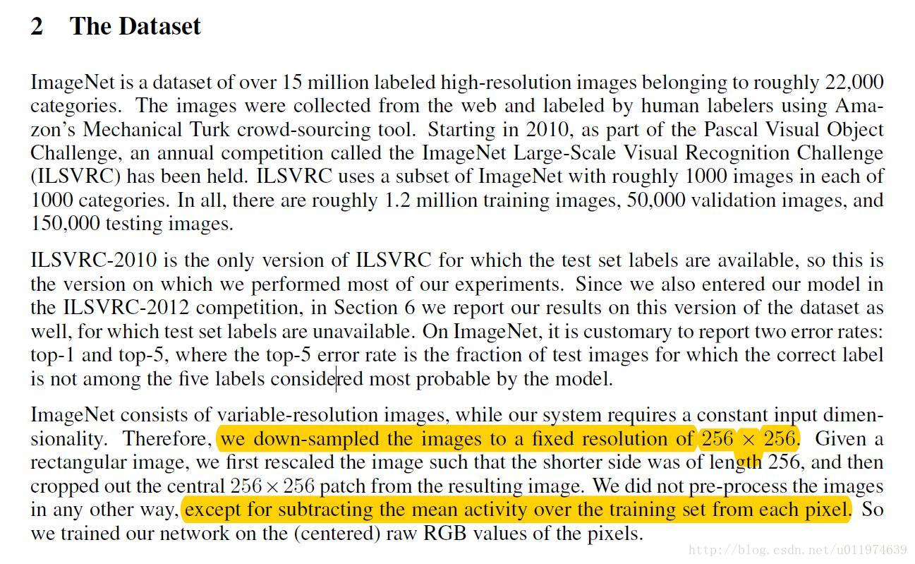
| we down-sampled the images to a fixed resolution of 256 x 256. except for subtracting the mean activity over the training set from each pixel. |
数据集的处理方式: 对图片做放缩,下采样得到标准矩形大小为256x256图像 输入图像做去均值操作(后续有详解) |
3. 网络架构
| 原文 | description |
|---|---|
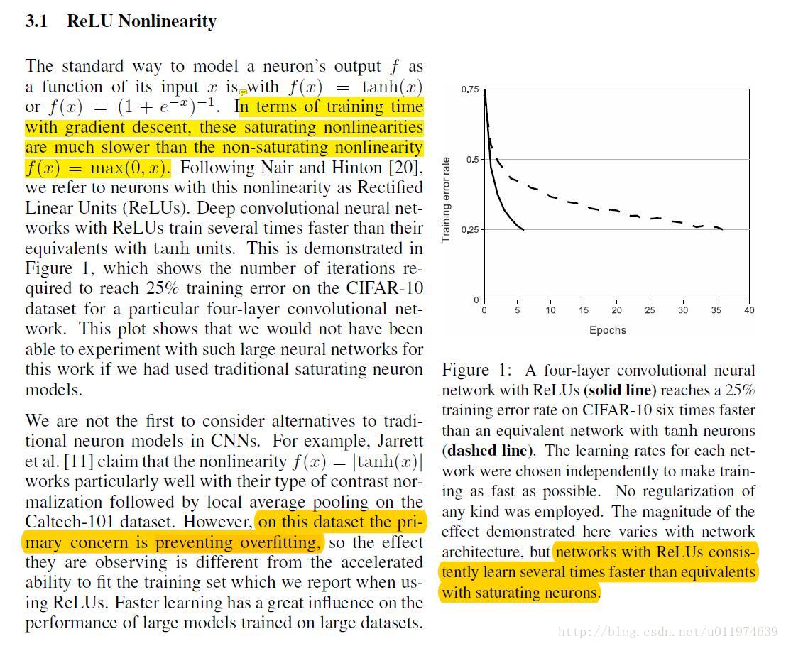
| In terms of training time with gradient descent, these saturating nonlinearities are much slower than the non-saturating nonlinearity f(x) = max(0, x). but networks with ReLUs consistently learn several times faster than equivalents with saturating neurons. on this dataset the primary concern is preventing overfitting |
ReLU激活函数的应用: 传统的激活函数,例如sigmoid或tanh会存在梯度弥散/消失问题,导致训练速度降低 以前的paper使用ReLU配置均值池化来防止过拟合,本文使用ReLU激活函数可以大幅度提高训练速度 |
注解
如图可以看到sigmoid、tanh函数存在饱和区,即在输入取较大或者较小值时,输出值饱和。这样的激活函数存在一个问题:在饱和区域,gradient较小,尤其是在深度网络中,会有gradient vanishing的问题,导致训练收敛速度降低。
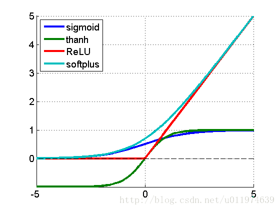
ReLU函数的特性决定了在大部分情况下,其gradient为常数,有利于BP的误差传递。
同时还有一个特性(个人见解):ReLU函数当输入小于等于零,输出也为零,这和dropout技术(下面有解释)有点相似,可以提高模型的鲁棒性。
当然,这里不是说ReLU就一定比sigmoid或tanh好,ReLU的不是全程可导(优势:ReLU的导数计算比sigmoid或tanh简单的多);ReLU的输出范围区间不可控。
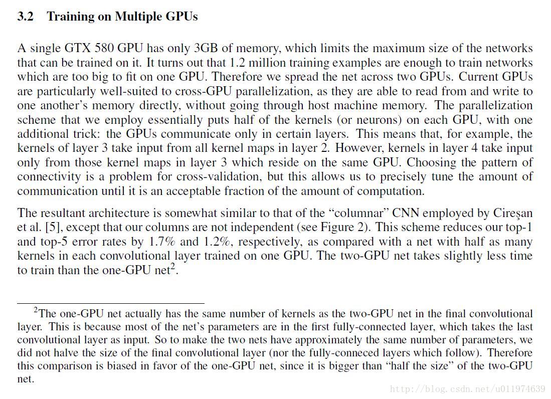
现在GPU单卡的计算力和显存可以放下整个AlexNet了,这里就不过分讨论论文里关于使用多GPU加速计算的内容了
| 原文 | description |
|---|---|
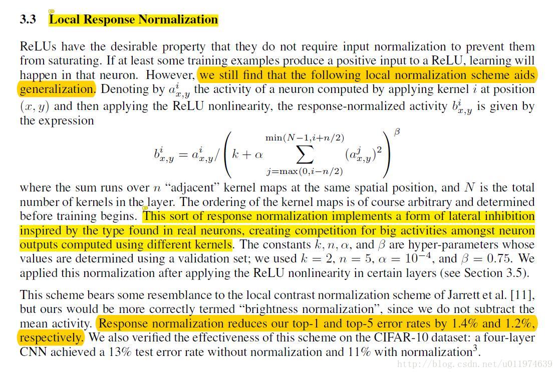
| we still find that the following local normalization scheme aids generalization. This sort of response normalization implements a form of lateral inhibition inspired by the type found in real neurons, creating competition for big activities amongst neuron outputs computed using different kernels. Response normalization reduces our top-1 and top-5 error rates by 1.4% and 1.2%, respectively. |
论文有关于局部响应归一化的看法: 在ReLU后,做LRN处理可以提高模型的泛化能力 LRN处理类似于生物神经元的横向抑制机制,可以理解为将局部响应最大的再放大,并抑制其他响应较小的(我的理解这是放大局部显著特征,作用还是提高鲁棒性) 在AlexNet中加LRN层可以降低错误率(在下一篇VGGNet论文中实验指出LRN并不能降低错误率,反倒加大了计算量,LRN的应用场合还需要再考量) |
| 原文 | description |
|---|---|
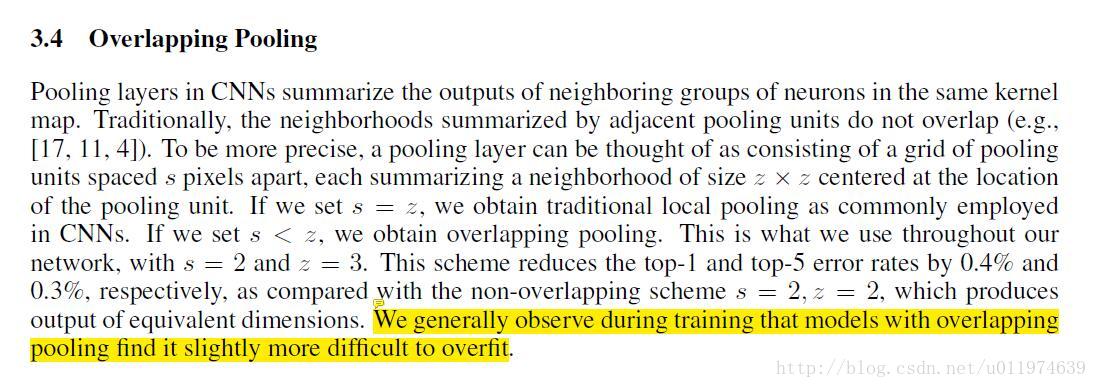
| each summarizing a neighborhood of size z * z centered at the location of the pooling unit. If we set s < z, we obtain overlapping pooling We generally observe during training that models with overlapping pooling find it slightly more difficult to overfit. |
重叠最大池化层的使用: 池化核的大小为z * z,如果移动的步长s < z,就得到了重叠的池化结果 使用重叠的池化层可以增强模型提取特征的能力,有利于防止过拟合 |

| 原文 | description |
|---|---|
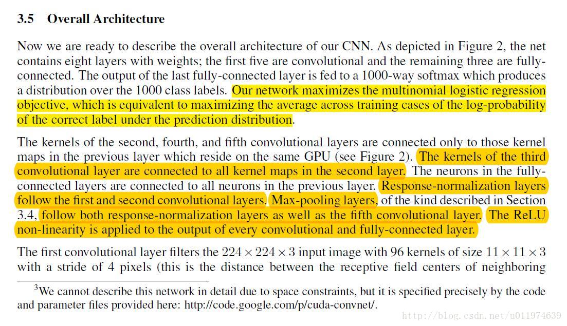
| Our network maximizes the multinomial logistic regression objective, which is equivalent to maximizing the average across training cases of the log-probability of the correct label under the prediction distribution. The neurons in the fully connected layers are connected to all neurons in the previous layer. Response-normalization layers follow the first and second convolutional layers. Max-pooling layers follow both response-normalization layers as well as the fifth convolutional layer. The ReLU non-linearity is applied to the output of every convolutional and fully-connected layer. The third, fourth, and fifth convolutional layers are connected to one another without any intervening pooling or normalization layers. |
详解介绍的一下网络架构: 网络最大化了多项logistic回归目标,等同于在预测分布下最大化了训练样本中正确标签的对数概率的平均值(softmax定义) FC层与上一层是全连接的,包括第五层卷积层输出与FC一层也是全连接的;第一层卷积和第二层卷积后有LRN层,再跟最大池化层 每一个卷积层后都做ReLU处理,第一第二卷积层后的LRN层也是处理ReLU的输出 第三层/第四层和第五层卷积层只单单做卷积,没有池化或LRN层 |
注解
(下面使用的结构与AlexNet类似,不全相同(AlexNet分GPU训练,连接方式不同))
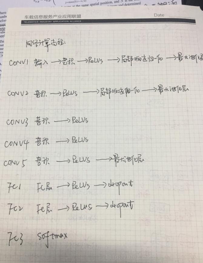
AlexNet的网络计算流程如下图:
| 连接层 | 计算流程 |
|---|---|
| 第一卷积层 | 输入–>卷积–>ReLUs–>LRN–>max-pooling |
| 第二卷积层 | 卷积–>ReLUs–>LRN–>max-pooling |
| 第三卷积层 | 卷积–>ReLUs |
| 第四卷积层 | 卷积–>ReLUs |
| 第五卷积层 | 卷积–>ReLUs |
| 第一全连接层 | 矩阵乘法–>ReLUs–>dropout(后面会介绍) |
| 第二全连接层 | 矩阵乘法–>ReLUs–>dropout |
| 第三全连接层(softmax层) | 矩阵乘法–>ReLUs–>softmax |
整体的计算架构(简化了ReLU、LRN、Dropout等操作)如下:
| 操作层 | 结果 | 操作步骤 |
|---|---|---|
| INPUT | [227x227x3] | 注:论文标准是224(实际计算应该是227) |
| CONV1 | [55x55x96] | 96 11x11 filters at stride 4, pad 0 (227-11)/4 + 1 = 55 |
| MAX POOL1 | [27x27x96] | 3x3 filters at stride 2 (55-3)/2 + 1 = 27 |
| CONV2 | [27x27x256] | 256 5x5 filters at stride 1, pad 2 (27-5 + 2*2)/1 + 1 = 27 |
| MAX POOL2 | [13x13x256] | 3x3 filters at stride 2 (27 -3)/2 + 1 = 13 |
| CONV3 | [13x13x384] | 384 3x3 filters at stride 1, pad 1 (13-3 + 2*1)/1 + 1 = 13 |
| CONV4 | [13x13x384] | 384 3x3 filters at stride 1, pad 1 (13-3 + 2*1)/1 + 1 = 13 |
| CONV5 | [13x13x256] | 256 3x3 filters at stride 1, pad 1 (13-3 + 2*1)/1 + 1 = 13 |
| MAX POOL3 | [6x6x256] | 3x3 filters at stride 2 (13-3)/2 + 1 = 6 |
| FC1 | [4096] | 4096 neurons |
| FC2 | [4096] | 4096 neurons |
| SOFTMAX | [1000] | 1000 neurons |
模型使用的资源如下:
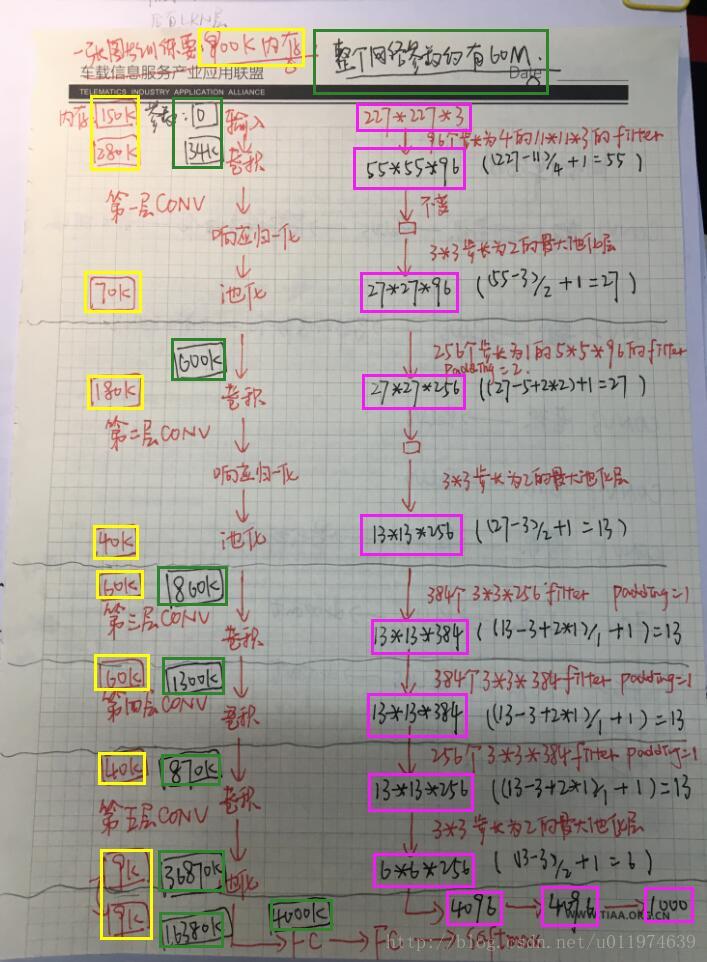
| 连接层 | 参数量 | 占用显存量(GPU训练一张图片) |
|---|---|---|
| 第一卷积层 | 34K | 500K |
| 第二卷积层 | 600K | 220K |
| 第三卷积层 | 860K | 60K |
| 第四卷积层 | 1300K | 60K |
| 第五卷积层 | 870K | 49K |
| 第一全连接层 | 36870K | 4K |
| 第二全连接层 | 16380K | 4K |
| 第三全连接层(softmax层) | 4000K | 1K |
| 合计 | 一张图片:60M*4bytes = 240M | 900K |
4. 减少过拟合
| 原文 | description |
|---|---|
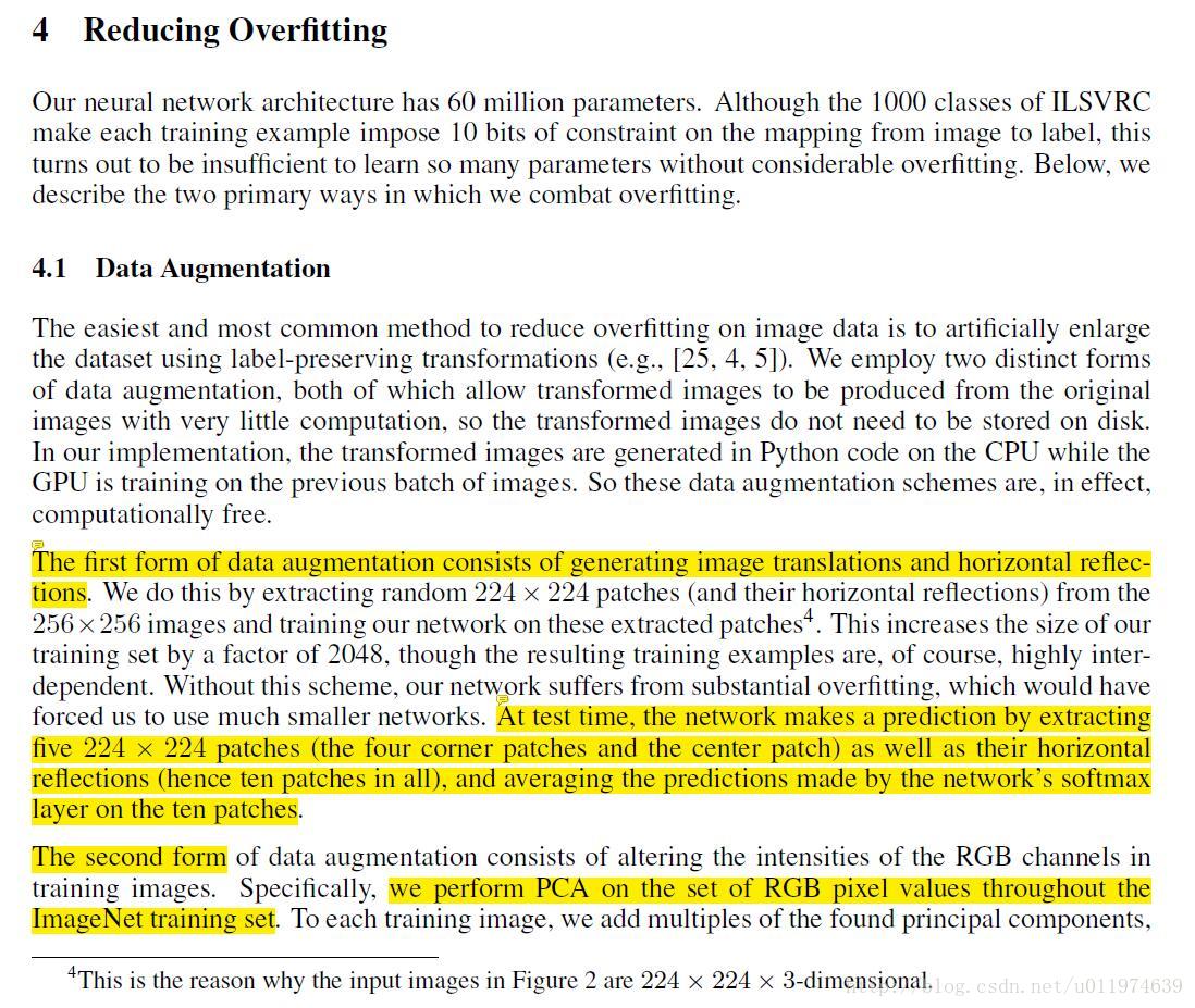
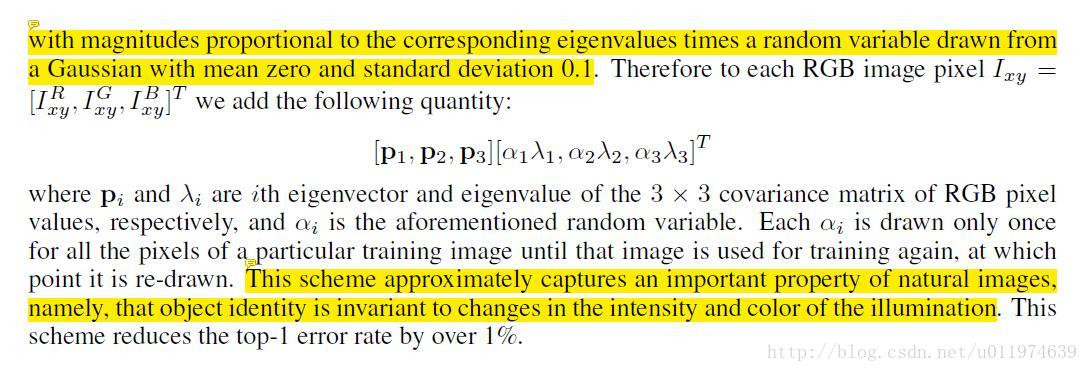
| The first form of data augmentation consists of generating image translations and horizontal reflections. This increases the size of our training set by a factor of 2048, though the resulting training examples are, of course, highly interdependent. At test time, the network makes a prediction by extracting five 224 * 224 patches (the four corner patches and the center patch) as well as their horizontal reflections (hence ten patches in all), and averaging the predictions made by the network’s softmax layer on the ten patches. The second form of data augmentation consists of altering the intensities of the RGB channels in training images. Specifically, we perform PCA on the set of RGB pixel values throughout the ImageNet training set. To each training image, we add multiples of the found principal components,with magnitudes proportional to the corresponding eigenvalues times a random variable drawn from a Gaussian with mean zero and standard deviation 0.1. This scheme approximately captures an important property of natural images, namely, that object identity is invariant to changes in the intensity and color of the illumination. |
有关于减少过拟合现象的操作: 第一种方式:数据增强 通过随机截取输入中固定大小的图片,并做水平翻转,扩大数据集,减少过拟合情况 数据集可扩大到原来的2048倍 (256-224)^2 * 2 = 2048 在做预测时,取出测试图片的十张patch(四角+中间,再翻转)作为输入,十张patch在softmax层输出相加去平均值作为最后的输出结果 第二种方式:改变训练图片的RGB通道值 对原训练集做PCA(主成分分析),对每一张训练图片,加上多倍的主成分 (个人理解:这样操作类似于信号处理中的去均值,消除直流分量的影响) 经过做PCA分析的处理,减少了模型的过拟合现象。可以得到一个自然图像的性质,改变图像的光照的颜色和强度,目标的特性是不变的,并且这样的处理有利于减少过拟合。 |
| 原文 | description |
|---|---|
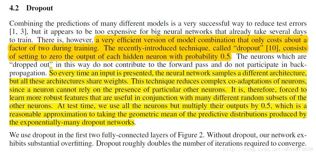
| a very efficient version of model combination that only costs about a factor of two during training. The recently-introduced technique, called “dropout” [10], consists of setting to zero the output of each hidden neuron with probability 0.5. every time an input is presented, the neural network samples a different architecture, but all these architectures share weights. This technique reduces complex co-adaptations of neurons, since a neuron cannot rely on the presence of particular other neurons. It is, therefore, forced to learn more robust features that are useful in conjunction with many different random subsets of the other neurons. we use all the neurons but multiply their outputs by 0.5, which is a reasonable approximation to taking the geometric mean of the predictive distributions produced by the exponentially-many dropout networks. |
使用dropout减少过拟合现象: dropout技术即让hidden层的神经元以50%的概率参与前向传播和反向传播. dropout技术减少了神经元之间的耦合,在每一次传播的过程中,hidden层的参与传播的神经元不同,整个模型的网络就不相同了,这样就会强迫网络学习更robust的特征,从而提高了模型的鲁棒性 对采用dropout技术的层,在输出时候要乘以0.5,这是一个合理的预测分布下的几何平均数的近似 |
5. 训练细节

| 原文 | description |
|---|---|
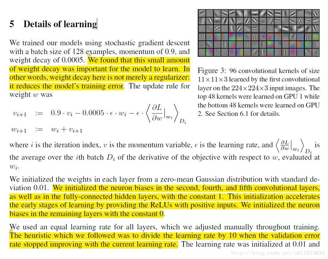
| We found that this small amount of weight decay was important for the model to learn. In other words, weight decay here is not merely a regularizer: it reduces the model’s training error. We initialized the neuron biases in the second, fourth, and fifth convolutional layers, as well as in the fully-connected hidden layers, with the constant 1. This initialization accelerates the early stages of learning by providing the ReLUs with positive inputs. We initialized the neuron biases in the remaining layers with the constant 0. The heuristic which we followed was to divide the learning rate by 10 when the validation error rate stopped improving with the current learning rate |
在训练调试上的细节描述: 使用小幅度的权值衰减,很利于模型的训练学习 对于第二、第四、第五卷积层还有全连接层,我们将bias初始化为1,有利于给ReLU提供一个正输入,加快训练速度 ;剩下的层bias初始化为0 学习率我们初始化为0.01,当模型在验证集错误率不提升时,我们将学习率降低10倍,整个训练过程降低了三次 |
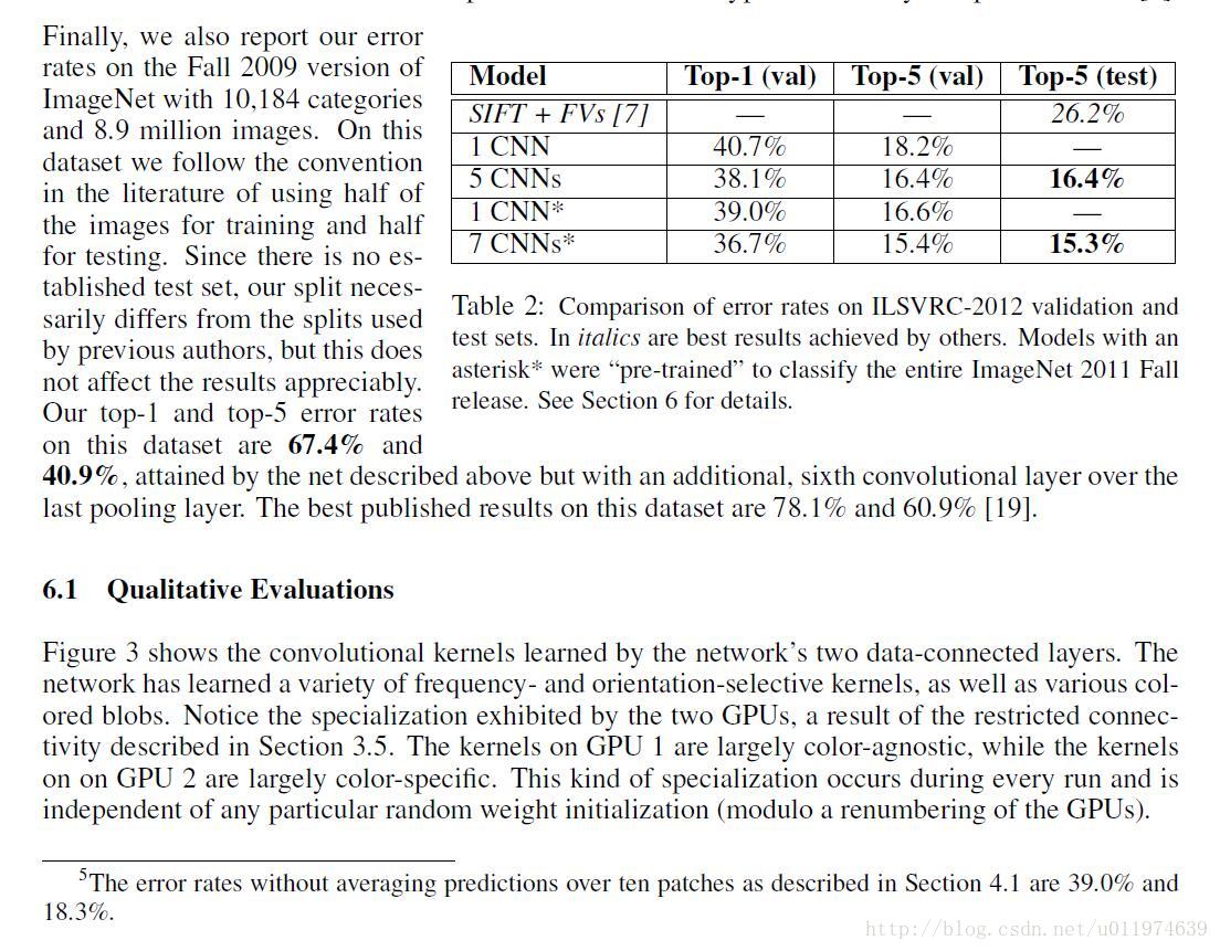
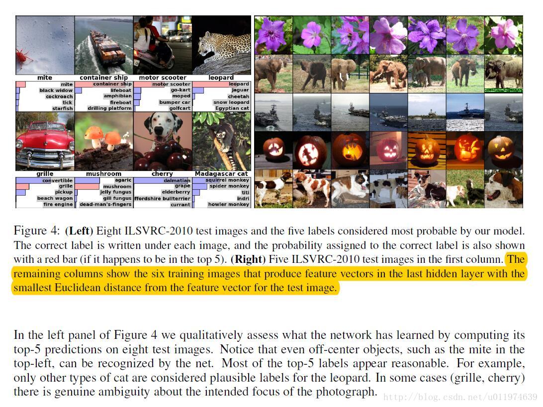
6. 结果
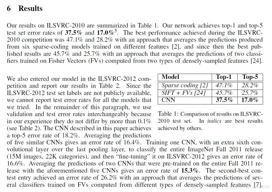
| 原文 | description |
|---|---|
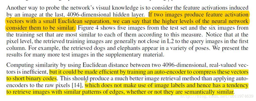
| The remaining columns show the six training images that produce feature vectors in the last hidden layer with the smallest Euclidean distance from the feature vector for the test image. If two images produce feature activation vectors with a small Euclidean separation, we can say that the higher levels of the neural network consider them to be similar. |
模型结果的分析: 图片右边展示了和测试图片在输出层上向量欧式距离很小的几张图片,可以看到这几张图片非常相似 我们可以得出结论,在特征激活向量的欧式距离相差较小的话,可以认为两张图片非常相似 |
7. 讨论
参考文献(略…)
AlexNet在TensorFlow里面实现
TensorFlow官方给出的AlexNet实现
首先给出的是TensorFlow官方的AlexNet实现,因为ImageNet数据集太大,所以官方是代码实现计算了前向和反向的训练时间,并没有真正的训练模型。其后,我在MNIST和CIFAR10上测试了AlexNet的性能。
实现代码
源代码在
models.tutorials.image.alexnet.alexnet_benchmark.py
- 1
实际代码如下:
# coding:utf8
# Copyright 2015 The TensorFlow Authors. All Rights Reserved.
#
# Licensed under the Apache License, Version 2.0 (the "License");
# you may not use this file except in compliance with the License.
# You may obtain a copy of the License at
#
#     http://www.apache.org/licenses/LICENSE-2.0
#
# Unless required by applicable law or agreed to in writing, software
# distributed under the License is distributed on an "AS IS" BASIS,
# WITHOUT WARRANTIES OR CONDITIONS OF ANY KIND, either express or implied.
# See the License for the specific language governing permissions and
# limitations under the License.
# ==============================================================================


"""Timing benchmark for AlexNet inference.

To run, use:
  bazel run -c opt --config=cuda \
      models/tutorials/image/alexnet:alexnet_benchmark

Across 100 steps on batch size = 128.

Forward pass:
Run on Tesla K40c: 145 +/- 1.5 ms / batch
Run on Titan X:     70 +/- 0.1 ms / batch

Forward-backward pass:
Run on Tesla K40c: 480 +/- 48 ms / batch
Run on Titan X:    244 +/- 30 ms / batch
"""
from __future__ import absolute_import
from __future__ import division
from __future__ import print_function

import argparse
from datetime import datetime
import math
import sys
import time

from six.moves import xrange  # pylint: disable=redefined-builtin
import tensorflow as tf

FLAGS = None


def print_activations(t):
  '''
    展示一个Tensor的name和shape
  :param t:
  :return:
  '''
  print(t.op.name, ' ', t.get_shape().as_list())


def inference(images):
  '''
   定义了AlexNet的前五个卷积层(FC计算速度较快,这里不做考虑)
  :param images: 输入图像Tensor
  :return:  返回最后一层pool5和parameters
  '''
  parameters = []

  # conv1
  # 使用name_scope可以将scope内创建的Variable命名conv1/xxx,便于区分不同卷积层的参数
  # 64个卷积核为11*11*3,步长为4,初始化权值为截断的正态分布(标注差为0.1)
  with tf.name_scope('conv1') as scope:
    kernel = tf.Variable(tf.truncated_normal([11, 11, 3, 64], dtype=tf.float32,
                                             stddev=1e-1), name='weights')
    conv = tf.nn.conv2d(images, kernel, [1, 4, 4, 1], padding='SAME')
    biases = tf.Variable(tf.constant(0.0, shape=[64], dtype=tf.float32),
                         trainable=True, name='biases')
    bias = tf.nn.bias_add(conv, biases)
    conv1 = tf.nn.relu(bias, name=scope)
    print_activations(conv1)
    parameters += [kernel, biases]

  # lrn1
  #
  with tf.name_scope('lrn1') as scope:
    lrn1 = tf.nn.lrn(conv1, alpha=1e-4, beta=0.75, depth_radius=2, bias=2.0)

  # pool1
  # 池化核3*3 步长为2*2
  pool1 = tf.nn.max_pool(lrn1, ksize=[1, 3, 3, 1], strides=[1, 2, 2, 1], padding='VALID')
  print_activations(pool1)

  # conv2
  # 192个卷积核为5*5*64,步长为1,初始化权值为截断的正态分布(标注差为0.1)
  with tf.name_scope('conv2') as scope:
    kernel = tf.Variable(tf.truncated_normal([5, 5, 64, 192], dtype=tf.float32,
                                             stddev=1e-1), name='weights')
    conv = tf.nn.conv2d(pool1, kernel, [1, 1, 1, 1], padding='SAME')
    biases = tf.Variable(tf.constant(0.0, shape=[192], dtype=tf.float32),
                         trainable=True, name='biases')
    bias = tf.nn.bias_add(conv, biases)
    conv2 = tf.nn.relu(bias, name=scope)
    parameters += [kernel, biases]
  print_activations(conv2)

  # lrn2
  with tf.name_scope('lrn2') as scope:
    lrn2 = tf.nn.lrn(conv2, alpha=1e-4, beta=0.75, depth_radius=2, bias=2.0)

  # pool2
  pool2 = tf.nn.max_pool(lrn2, ksize=[1, 3, 3, 1], strides=[1, 2, 2, 1], padding='VALID')
  print_activations(pool2)

  # conv3
  # 384个卷积核为3*3*192,步长为1,初始化权值为截断的正态分布(标注差为0.1)
  with tf.name_scope('conv3') as scope:
    kernel = tf.Variable(tf.truncated_normal([3, 3, 192, 384],
                                             dtype=tf.float32,
                                             stddev=1e-1), name='weights')
    conv = tf.nn.conv2d(pool2, kernel, [1, 1, 1, 1], padding='SAME')
    biases = tf.Variable(tf.constant(0.0, shape=[384], dtype=tf.float32),
                         trainable=True, name='biases')
    bias = tf.nn.bias_add(conv, biases)
    conv3 = tf.nn.relu(bias, name=scope)
    parameters += [kernel, biases]
    print_activations(conv3)

  # conv4
  # 256个卷积核为3*3*384,步长为1,初始化权值为截断的正态分布(标注差为0.1)
  with tf.name_scope('conv4') as scope:
    kernel = tf.Variable(tf.truncated_normal([3, 3, 384, 256],
                                             dtype=tf.float32,
                                             stddev=1e-1), name='weights')
    conv = tf.nn.conv2d(conv3, kernel, [1, 1, 1, 1], padding='SAME')
    biases = tf.Variable(tf.constant(0.0, shape=[256], dtype=tf.float32),
                         trainable=True, name='biases')
    bias = tf.nn.bias_add(conv, biases)
    conv4 = tf.nn.relu(bias, name=scope)
    parameters += [kernel, biases]
    print_activations(conv4)

  # conv5
  # 256个卷积核为3*3*256,步长为1,初始化权值为截断的正态分布(标注差为0.1)
  with tf.name_scope('conv5') as scope:
    kernel = tf.Variable(tf.truncated_normal([3, 3, 256, 256],
                                             dtype=tf.float32,
                                             stddev=1e-1), name='weights')
    conv = tf.nn.conv2d(conv4, kernel, [1, 1, 1, 1], padding='SAME')
    biases = tf.Variable(tf.constant(0.0, shape=[256], dtype=tf.float32),
                         trainable=True, name='biases')
    bias = tf.nn.bias_add(conv, biases)
    conv5 = tf.nn.relu(bias, name=scope)
    parameters += [kernel, biases]
    print_activations(conv5)

  # pool5
  pool5 = tf.nn.max_pool(conv5, ksize=[1, 3, 3, 1], strides=[1, 2, 2, 1], padding='VALID')
  print_activations(pool5)

  return pool5, parameters


def time_tensorflow_run(session, target, info_string):
  '''
    用于评估AlexNet计算时间
  :param session:
  :param target:
  :param info_string:
  :return:
  '''
  num_steps_burn_in = 10  # 设备热身,存在显存加载/cache命中等问题
  total_duration = 0.0      # 总时间
  total_duration_squared = 0.0  # 用于计算方差

  for i in xrange(FLAGS.num_batches + num_steps_burn_in):
    start_time = time.time()
    _ = session.run(target)
    duration = time.time() - start_time
    if i >= num_steps_burn_in:
      if not i % 10:
        print ('%s: step %d, duration = %.3f' %
               (datetime.now(), i - num_steps_burn_in, duration))
      total_duration += duration
      total_duration_squared += duration * duration

  mn = total_duration / FLAGS.num_batches
  vr = total_duration_squared / FLAGS.num_batches - mn * mn
  sd = math.sqrt(vr)
  print ('%s: %s across %d steps, %.3f +/- %.3f sec / batch' %
         (datetime.now(), info_string, FLAGS.num_batches, mn, sd))


def run_benchmark():
  '''
    随机生成一张图片,
  :return:
  '''
  with tf.Graph().as_default():
    # Generate some dummy images.
    image_size = 224
    # Note that our padding definition is slightly different the cuda-convnet.
    # In order to force the model to start with the same activations sizes,
    # we add 3 to the image_size and employ VALID padding above.
    images = tf.Variable(tf.random_normal([FLAGS.batch_size,
                                           image_size,
                                           image_size, 3],
                                          dtype=tf.float32,
                                          stddev=1e-1))

    # Build a Graph that computes the logits predictions from the
    # inference model.
    pool5, parameters = inference(images)

    # Build an initialization operation.
    init = tf.global_variables_initializer()

    # Start running operations on the Graph.
    config = tf.ConfigProto()
    config.gpu_options.allocator_type = 'BFC'
    sess = tf.Session(config=config)
    sess.run(init)

    # Run the forward benchmark.
    time_tensorflow_run(sess, pool5, "Forward")

    # Add a simple objective so we can calculate the backward pass.
    objective = tf.nn.l2_loss(pool5)
    # Compute the gradient with respect to all the parameters.
    grad = tf.gradients(objective, parameters)  #计算梯度(objective与parameters有相关)
    # Run the backward benchmark.
    time_tensorflow_run(sess, grad, "Forward-backward")


def main(_):
  run_benchmark()


if __name__ == '__main__':
  parser = argparse.ArgumentParser()
  parser.add_argument(
      '--batch_size',
      type=int,
      default=128,
      help='Batch size.'
  )
  parser.add_argument(
      '--num_batches',
      type=int,
      default=100,
      help='Number of batches to run.'
  )
  FLAGS, unparsed = parser.parse_known_args()
  tf.app.run(main=main, argv=[sys.argv[0]] + unparsed)
- 1
- 2
- 3
- 4
- 5
- 6
- 7
- 8
- 9
- 10
- 11
- 12
- 13
- 14
- 15
- 16
- 17
- 18
- 19
- 20
- 21
- 22
- 23
- 24
- 25
- 26
- 27
- 28
- 29
- 30
- 31
- 32
- 33
- 34
- 35
- 36
- 37
- 38
- 39
- 40
- 41
- 42
- 43
- 44
- 45
- 46
- 47
- 48
- 49
- 50
- 51
- 52
- 53
- 54
- 55
- 56
- 57
- 58
- 59
- 60
- 61
- 62
- 63
- 64
- 65
- 66
- 67
- 68
- 69
- 70
- 71
- 72
- 73
- 74
- 75
- 76
- 77
- 78
- 79
- 80
- 81
- 82
- 83
- 84
- 85
- 86
- 87
- 88
- 89
- 90
- 91
- 92
- 93
- 94
- 95
- 96
- 97
- 98
- 99
- 100
- 101
- 102
- 103
- 104
- 105
- 106
- 107
- 108
- 109
- 110
- 111
- 112
- 113
- 114
- 115
- 116
- 117
- 118
- 119
- 120
- 121
- 122
- 123
- 124
- 125
- 126
- 127
- 128
- 129
- 130
- 131
- 132
- 133
- 134
- 135
- 136
- 137
- 138
- 139
- 140
- 141
- 142
- 143
- 144
- 145
- 146
- 147
- 148
- 149
- 150
- 151
- 152
- 153
- 154
- 155
- 156
- 157
- 158
- 159
- 160
- 161
- 162
- 163
- 164
- 165
- 166
- 167
- 168
- 169
- 170
- 171
- 172
- 173
- 174
- 175
- 176
- 177
- 178
- 179
- 180
- 181
- 182
- 183
- 184
- 185
- 186
- 187
- 188
- 189
- 190
- 191
- 192
- 193
- 194
- 195
- 196
- 197
- 198
- 199
- 200
- 201
- 202
- 203
- 204
- 205
- 206
- 207
- 208
- 209
- 210
- 211
- 212
- 213
- 214
- 215
- 216
- 217
- 218
- 219
- 220
- 221
- 222
- 223
- 224
- 225
- 226
- 227
- 228
- 229
- 230
- 231
- 232
- 233
- 234
- 235
- 236
- 237
- 238
- 239
- 240
- 241
- 242
- 243
- 244
- 245
- 246
- 247
- 248
- 249
- 250
- 251
- 252
- 253
- 254
- 255
输出
带LRN层的计算时间:
2017-07-28 20:01:13.982322: step 0, duration = 0.095
2017-07-28 20:01:14.926004: step 10, duration = 0.093
2017-07-28 20:01:15.873614: step 20, duration = 0.094
2017-07-28 20:01:16.820571: step 30, duration = 0.095
2017-07-28 20:01:17.770994: step 40, duration = 0.095
2017-07-28 20:01:18.717510: step 50, duration = 0.095
2017-07-28 20:01:19.664164: step 60, duration = 0.094
2017-07-28 20:01:20.614472: step 70, duration = 0.094
2017-07-28 20:01:21.556516: step 80, duration = 0.094
2017-07-28 20:01:22.497904: step 90, duration = 0.094
2017-07-28 20:01:23.360716: Forward across 100 steps, 0.095 +/- 0.001 sec / batch
2017-07-28 20:01:26.080152: step 0, duration = 0.216
2017-07-28 20:01:28.242078: step 10, duration = 0.216
2017-07-28 20:01:30.418645: step 20, duration = 0.217
2017-07-28 20:01:32.583144: step 30, duration = 0.216
2017-07-28 20:01:34.748482: step 40, duration = 0.216
2017-07-28 20:01:36.916634: step 50, duration = 0.216
2017-07-28 20:01:39.073233: step 60, duration = 0.215
2017-07-28 20:01:41.233626: step 70, duration = 0.217
2017-07-28 20:01:43.395616: step 80, duration = 0.216
2017-07-28 20:01:45.557092: step 90, duration = 0.216
2017-07-28 20:01:47.502201: Forward-backward across 100 steps, 0.216 +/- 0.001 sec / batch


不带LRN层的计算时间:
2017-07-28 20:03:44.466247: step 0, duration = 0.035
2017-07-28 20:03:44.812274: step 10, duration = 0.034
2017-07-28 20:03:45.158224: step 20, duration = 0.034
2017-07-28 20:03:45.503790: step 30, duration = 0.034
2017-07-28 20:03:45.849637: step 40, duration = 0.034
2017-07-28 20:03:46.195617: step 50, duration = 0.035
2017-07-28 20:03:46.541352: step 60, duration = 0.034
2017-07-28 20:03:46.886702: step 70, duration = 0.035
2017-07-28 20:03:47.232510: step 80, duration = 0.034
2017-07-28 20:03:47.576873: step 90, duration = 0.035
2017-07-28 20:03:47.886823: Forward across 100 steps, 0.035 +/- 0.000 sec / batch
2017-07-28 20:03:49.313215: step 0, duration = 0.099
2017-07-28 20:03:50.310755: step 10, duration = 0.100
2017-07-28 20:03:51.306087: step 20, duration = 0.099
2017-07-28 20:03:52.302013: step 30, duration = 0.100
2017-07-28 20:03:53.296832: step 40, duration = 0.100
2017-07-28 20:03:54.295764: step 50, duration = 0.100
2017-07-28 20:03:55.293681: step 60, duration = 0.100
2017-07-28 20:03:56.292695: step 70, duration = 0.100
2017-07-28 20:03:57.291794: step 80, duration = 0.100
2017-07-28 20:03:58.289415: step 90, duration = 0.100
2017-07-28 20:03:59.187312: Forward-backward across 100 steps, 0.100 +/- 0.000 sec / batch
- 1
- 2
- 3
- 4
- 5
- 6
- 7
- 8
- 9
- 10
- 11
- 12
- 13
- 14
- 15
- 16
- 17
- 18
- 19
- 20
- 21
- 22
- 23
- 24
- 25
- 26
- 27
- 28
- 29
- 30
- 31
- 32
- 33
- 34
- 35
- 36
- 37
- 38
- 39
- 40
- 41
- 42
- 43
- 44
- 45
- 46
- 47
- 48
- 49
可以看到不带LRN的计算速度提高了近三倍,且带LRN层对模型的影响不够明显。实际实现过程中考量计算资源和计算时间,选择是否使用LRN层
AlexNet应用在MNIST数据集上
因为MNIST数据集的图片展开为28*28*1,数据集上图片都较小,所有我们在卷积层和池化层的操作上都缩小了操作核的大小和步长,以保持图像的尺寸不会迅速崩塌。
实现代码
这里实现的是简化版的AlexNet,在卷积层上缩小了卷积了,移动步长也都改为了1,池化层都使用了2*2,且移动步长也改为了1
# coding=utf-8
import tensorflow as tf
from tensorflow.examples.tutorials.mnist import input_data


STEPS = 1500
batch_size = 64

mnist = input_data.read_data_sets('MNIST_data', one_hot=True)


parameters = {
    'w1': tf.Variable(tf.truncated_normal([3, 3, 1, 64], dtype=tf.float32, stddev=1e-1), name='w1'),
    'w2': tf.Variable(tf.truncated_normal([3, 3, 64, 64], dtype=tf.float32, stddev=1e-1), name='w2'),
    'w3': tf.Variable(tf.truncated_normal([3, 3, 64, 128], dtype=tf.float32, stddev=1e-1), name='w3'),
    'w4': tf.Variable(tf.truncated_normal([3, 3, 128, 128], dtype=tf.float32, stddev=1e-1), name='w4'),
    'w5': tf.Variable(tf.truncated_normal([3, 3, 128, 256], dtype=tf.float32, stddev=1e-1), name='w5'),
    'fc1': tf.Variable(tf.truncated_normal([256*28*28, 1024], dtype=tf.float32, stddev=1e-2), name='fc1'),
    'fc2': tf.Variable(tf.truncated_normal([1024, 1024], dtype=tf.float32, stddev=1e-2), name='fc2'),
    'softmax': tf.Variable(tf.truncated_normal([1024, 10], dtype=tf.float32, stddev=1e-2), name='fc3'),
    'bw1': tf.Variable(tf.random_normal([64])),
    'bw2': tf.Variable(tf.random_normal([64])),
    'bw3': tf.Variable(tf.random_normal([128])),
    'bw4': tf.Variable(tf.random_normal([128])),
    'bw5': tf.Variable(tf.random_normal([256])),
    'bc1': tf.Variable(tf.random_normal([1024])),
    'bc2': tf.Variable(tf.random_normal([1024])),
    'bs': tf.Variable(tf.random_normal([10]))
}

def conv2d(_x, _w, _b):
    '''
         封装的生成卷积层的函数
         因为NNIST的图片较小,这里采用1,1的步长
    :param _x:  输入
    :param _w:  卷积核
    :param _b:  bias
    :return:    卷积操作
    '''
    return tf.nn.relu(tf.nn.bias_add(tf.nn.conv2d(_x, _w, [1, 1, 1, 1], padding='SAME'), _b))

def lrn(_x):
    '''
    作局部响应归一化处理
    :param _x:
    :return:
    '''
    return tf.nn.lrn(_x, depth_radius=4, bias=1.0, alpha=0.001 / 9.0, beta=0.75)

def max_pool(_x, f):
    '''
        最大池化处理,因为输入图片尺寸较小,这里取步长固定为1,1,1,1
    :param _x:
    :param f:
    :return:
    '''
    return tf.nn.max_pool(_x, [1, f, f, 1], [1, 1, 1, 1], padding='SAME')

def inference(_parameters,_dropout):
    '''
     定义网络结构和训练过程
    :param _parameters:  网络结构参数
    :param _dropout:     dropout层的keep_prob
    :return:
    '''

    # 搭建Alex模型
    x = tf.placeholder(tf.float32, [None, 784]) # 输入: MNIST数据图像为展开的向量
    x_ = tf.reshape(x, shape=[-1, 28, 28, 1])   # 将训练数据reshape成单通道图片
    y_ = tf.placeholder(tf.float32, [None, 10]) # 标签值:one-hot标签值

    # 第一卷积层
    conv1 = conv2d(x_, _parameters['w1'], _parameters['bw1'])
    lrn1 = lrn(conv1)
    pool1 = max_pool(lrn1, 2)

    # 第二卷积层
    conv2 = conv2d(pool1, _parameters['w2'], _parameters['bw2'])
    lrn2 = lrn(conv2)
    pool2 = max_pool(lrn2, 2)

    # 第三卷积层
    conv3 = conv2d(pool2, _parameters['w3'], _parameters['bw3'])

    # 第四卷积层
    conv4 = conv2d(conv3, _parameters['w4'], _parameters['bw4'])

    # 第五卷积层
    conv5 = conv2d(conv4, _parameters['w5'], _parameters['bw5'])
    pool5 = max_pool(conv5, 2)

    # FC1层
    shape = pool5.get_shape() # 获取第五卷基层输出结构,并展开
    reshape = tf.reshape(pool5, [-1, shape[1].value*shape[2].value*shape[3].value])
    fc1 = tf.nn.relu(tf.matmul(reshape, _parameters['fc1']) + _parameters['bc1'])
    fc1_drop = tf.nn.dropout(fc1, keep_prob=_dropout)

    # FC2层
    fc2 = tf.nn.relu(tf.matmul(fc1_drop, _parameters['fc2']) + _parameters['bc2'])
    fc2_drop = tf.nn.dropout(fc2, keep_prob=_dropout)

    # softmax层
    y_conv = tf.nn.softmax(tf.matmul(fc2_drop, _parameters['softmax']) + _parameters['bs'])

    # 定义损失函数和优化器
    cross_entropy = tf.reduce_mean(-tf.reduce_sum(y_ * tf.log(y_conv), reduction_indices=[1]))
    train_step = tf.train.AdamOptimizer(1e-4).minimize(cross_entropy)

    # 计算准确率
    correct_pred = tf.equal(tf.argmax(y_conv, 1), tf.argmax(y_, 1))
    accuracy = tf.reduce_mean(tf.cast(correct_pred, tf.float32))

    with tf.Session() as sess:
        initop = tf.global_variables_initializer()
        sess.run(initop)

        for step in range(STEPS):
            batch_xs, batch_ys = mnist.train.next_batch(batch_size)
            sess.run(train_step, feed_dict={x: batch_xs, y_: batch_ys})

            if step % 50 == 0:
                acc = sess.run(accuracy, feed_dict={x: batch_xs, y_: batch_ys})
                loss = sess.run(cross_entropy, feed_dict={x: batch_xs, y_: batch_ys})
                print('step:%5d. --acc:%.6f. -- loss:%.6f.'%(step, acc, loss))

        print('train over!')

        # Test
        test_xs, test_ys = mnist.test.images[:512], mnist.test.labels[:512]

        print('test acc:%f' % (sess.run(accuracy, feed_dict={x: test_xs, y_: test_ys})))

if __name__ == '__main__':
    inference(parameters, 0.9)
- 1
- 2
- 3
- 4
- 5
- 6
- 7
- 8
- 9
- 10
- 11
- 12
- 13
- 14
- 15
- 16
- 17
- 18
- 19
- 20
- 21
- 22
- 23
- 24
- 25
- 26
- 27
- 28
- 29
- 30
- 31
- 32
- 33
- 34
- 35
- 36
- 37
- 38
- 39
- 40
- 41
- 42
- 43
- 44
- 45
- 46
- 47
- 48
- 49
- 50
- 51
- 52
- 53
- 54
- 55
- 56
- 57
- 58
- 59
- 60
- 61
- 62
- 63
- 64
- 65
- 66
- 67
- 68
- 69
- 70
- 71
- 72
- 73
- 74
- 75
- 76
- 77
- 78
- 79
- 80
- 81
- 82
- 83
- 84
- 85
- 86
- 87
- 88
- 89
- 90
- 91
- 92
- 93
- 94
- 95
- 96
- 97
- 98
- 99
- 100
- 101
- 102
- 103
- 104
- 105
- 106
- 107
- 108
- 109
- 110
- 111
- 112
- 113
- 114
- 115
- 116
- 117
- 118
- 119
- 120
- 121
- 122
- 123
- 124
- 125
- 126
- 127
- 128
- 129
- 130
- 131
- 132
- 133
- 134
输出:
1500次训练结果
step:    0. --acc:0.140625. -- loss:25.965401.
step:   50. --acc:0.187500. -- loss:2.211631.
step:  100. --acc:0.828125. -- loss:0.606436.
step:  150. --acc:0.796875. -- loss:0.576135.
step:  200. --acc:0.859375. -- loss:0.446622.
step:  250. --acc:0.859375. -- loss:0.334442.
step:  300. --acc:0.843750. -- loss:0.339411.
step:  350. --acc:0.937500. -- loss:0.272400.
step:  400. --acc:0.906250. -- loss:0.298700.
step:  450. --acc:0.984375. -- loss:0.104384.
step:  500. --acc:0.921875. -- loss:0.259755.
step:  550. --acc:0.968750. -- loss:0.091056.
step:  600. --acc:0.968750. -- loss:0.112438.
step:  650. --acc:0.968750. -- loss:0.102413.
step:  700. --acc:0.968750. -- loss:0.067934.
step:  750. --acc:0.968750. -- loss:0.107729.
step:  800. --acc:0.968750. -- loss:0.089720.
step:  850. --acc:1.000000. -- loss:0.055279.
step:  900. --acc:1.000000. -- loss:0.048994.
step:  950. --acc:0.953125. -- loss:0.098056.
step: 1000. --acc:0.984375. -- loss:0.056790.
step: 1050. --acc:0.984375. -- loss:0.063745.
step: 1100. --acc:0.937500. -- loss:0.172236.
step: 1150. --acc:1.000000. -- loss:0.022871.
step: 1200. --acc:0.968750. -- loss:0.044372.
step: 1250. --acc:0.968750. -- loss:0.043271.
step: 1300. --acc:0.984375. -- loss:0.034694.
step: 1350. --acc:0.968750. -- loss:0.031569.
step: 1400. --acc:0.968750. -- loss:0.088058.
step: 1450. --acc:0.984375. -- loss:0.037831.
train over!
test acc:0.986328
- 1
- 2
- 3
- 4
- 5
- 6
- 7
- 8
- 9
- 10
- 11
- 12
- 13
- 14
- 15
- 16
- 17
- 18
- 19
- 20
- 21
- 22
- 23
- 24
- 25
- 26
- 27
- 28
- 29
- 30
- 31
- 32
最终的准确率在98.6%,效果还算可以,在微调加一些其他的tricks应该还是能用的。
AlexNet应用在CIFAR10数据集上
CIFAR10数据集的图片展开为24*24*3,两个数据集上图片都较小,所有我们在卷积层和池化层的操作上都缩小了操作核的大小和步长,以保持图像的尺寸不会迅速崩塌。
同样的以为CIFAR10的数据图像也不大,所以还是用简化版本的AlexNet。
# coding=utf-8


from  __future__ import division

import tensorflow as tf
from models.tutorials.image.cifar10 import cifar10,cifar10_input
import  numpy as np


STEPS = 10000
batch_size =128

data_dir = '/tmp/cifar10_data/cifar-10-batches-bin'


parameters = {
    'w1': tf.Variable(tf.truncated_normal([3, 3, 3, 32], dtype=tf.float32, stddev=1e-1), name='w1'),
    'w2': tf.Variable(tf.truncated_normal([3, 3, 32, 64], dtype=tf.float32, stddev=1e-1), name='w2'),
    'w3': tf.Variable(tf.truncated_normal([3, 3, 64, 64], dtype=tf.float32, stddev=1e-1), name='w3'),
    'w4': tf.Variable(tf.truncated_normal([3, 3, 64, 256], dtype=tf.float32, stddev=1e-1), name='w4'),
    'w5': tf.Variable(tf.truncated_normal([3, 3, 256, 128], dtype=tf.float32, stddev=1e-1), name='w5'),
    'fc1': tf.Variable(tf.truncated_normal([128*24*24, 1024], dtype=tf.float32, stddev=1e-2), name='fc1'),
    'fc2': tf.Variable(tf.truncated_normal([1024, 1024], dtype=tf.float32, stddev=1e-2), name='fc2'),
    'softmax': tf.Variable(tf.truncated_normal([1024, 10], dtype=tf.float32, stddev=1e-2), name='fc3'),
    'bw1': tf.Variable(tf.random_normal([32])),
    'bw2': tf.Variable(tf.random_normal([64])),
    'bw3': tf.Variable(tf.random_normal([64])),
    'bw4': tf.Variable(tf.random_normal([256])),
    'bw5': tf.Variable(tf.random_normal([128])),
    'bc1': tf.Variable(tf.random_normal([1024])),
    'bc2': tf.Variable(tf.random_normal([1024])),
    'bs': tf.Variable(tf.random_normal([10]))
}

def conv2d(_x, _w, _b):
    '''
         封装的生成卷积层的函数
         因为NNIST的图片较小,这里采用1,1的步长
    :param _x:  输入
    :param _w:  卷积核
    :param _b:  bias
    :return:    卷积操作
    '''
    return tf.nn.relu(tf.nn.bias_add(tf.nn.conv2d(_x, _w, [1, 1, 1, 1], padding='SAME'), _b))

def lrn(_x):
    '''
    作局部响应归一化处理
    :param _x:
    :return:
    '''
    return tf.nn.lrn(_x, depth_radius=4, bias=1.0, alpha=0.001 / 9.0, beta=0.75)

def max_pool(_x, f):
    '''
        最大池化处理,因为输入图片尺寸较小,这里取步长固定为1,1,1,1
    :param _x:
    :param f:
    :return:
    '''
    return tf.nn.max_pool(_x, [1, f, f, 1], [1, 1, 1, 1], padding='SAME')

def loss(logits, labels):
    '''
    使用tf.nn.sparse_softmax_cross_entropy_with_logits将softmax和cross_entropy_loss计算合在一起
    并计算cross_entropy的均值添加到losses集合.以便于后面输出所有losses
    :param logits:
    :param labels:
    :return:
    '''
    labels = tf.cast(labels, tf.int64)
    cross_entropy = tf.nn.sparse_softmax_cross_entropy_with_logits(logits=logits,
                                                        labels=labels, name='cross_entropy_per_example')
    cross_entropy_mean = tf.reduce_mean(cross_entropy, name='cross_entropy')
    tf.add_to_collection('losses',cross_entropy_mean)

    return tf.add_n(tf.get_collection('losses'), name='total_loss')

def inference(_parameters,_dropout):
    '''
     定义网络结构和训练过程
    :param _parameters:  网络结构参数
    :param _dropout:     dropout层的keep_prob
    :return:
    '''

    images_train, labels_train = cifar10_input.distorted_inputs(data_dir=data_dir, batch_size=batch_size)
    images_test, labels_test = cifar10_input.inputs(eval_data=True, data_dir=data_dir, batch_size=batch_size)

    image_holder = tf.placeholder(tf.float32, [batch_size, 24, 24, 3])
    label_holder = tf.placeholder(tf.int32, [batch_size])


    # 第一卷积层
    conv1 = conv2d(image_holder, _parameters['w1'], _parameters['bw1'])
    lrn1 = lrn(conv1)
    pool1 = max_pool(lrn1, 2)

    # 第二卷积层
    conv2 = conv2d(pool1, _parameters['w2'], _parameters['bw2'])
    lrn2 = lrn(conv2)
    pool2 = max_pool(lrn2, 2)

    # 第三卷积层
    conv3 = conv2d(pool2, _parameters['w3'], _parameters['bw3'])

    # 第四卷积层
    conv4 = conv2d(conv3, _parameters['w4'], _parameters['bw4'])

    # 第五卷积层
    conv5 = conv2d(conv4, _parameters['w5'], _parameters['bw5'])
    pool5 = max_pool(conv5, 2)

    # FC1层
    shape = pool5.get_shape() # 获取第五卷基层输出结构,并展开
    reshape = tf.reshape(pool5, [-1, shape[1].value*shape[2].value*shape[3].value])
    fc1 = tf.nn.relu(tf.matmul(reshape, _parameters['fc1']) + _parameters['bc1'])
    fc1_drop = tf.nn.dropout(fc1, keep_prob=_dropout)

    # FC2层
    fc2 = tf.nn.relu(tf.matmul(fc1_drop, _parameters['fc2']) + _parameters['bc2'])
    fc2_drop = tf.nn.dropout(fc2, keep_prob=_dropout)

    # softmax层
    logits = tf.add(tf.matmul(fc2_drop, _parameters['softmax']),_parameters['bs'])
    losses = loss(logits, label_holder)
    train_op = tf.train.AdamOptimizer(1e-3).minimize(losses)

    top_k_op = tf.nn.in_top_k(logits, label_holder, 1)


    # 创建默认session,初始化变量
    sess = tf.InteractiveSession()
    tf.global_variables_initializer().run()

    # 启动图片增强线程队列
    tf.train.start_queue_runners()

    initop = tf.global_variables_initializer()
    sess.run(initop)

    for step in range(STEPS):
        batch_xs, batch_ys = sess.run([images_train, labels_train])
        _, loss_value = sess.run([train_op, losses], feed_dict={image_holder: batch_xs,
                                                                label_holder: batch_ys} )
        if step % 20 == 0:
            print('step:%5d. --lost:%.6f. '%(step, loss_value))
    print('train over!')

    num_examples = 10000
    import math
    num_iter = int(math.ceil(num_examples / batch_size))
    true_count = 0
    total_sample_count = num_iter * batch_size  # 除去不够一个batch的
    step = 0
    while step < num_iter:
        image_batch, label_batch = sess.run([images_test, labels_test])
        predictions = sess.run([top_k_op], feed_dict={image_holder: image_batch,
                                                      label_holder: label_batch})
        true_count += np.sum(predictions)  # 利用top_k_op计算输出结果
        step += 1

    precision = true_count / total_sample_count

    print('precision @ 1=%.3f' % precision)


if __name__ == '__main__':
    cifar10.maybe_download_and_extract()
    inference(parameters, 0.7)
- 1
- 2
- 3
- 4
- 5
- 6
- 7
- 8
- 9
- 10
- 11
- 12
- 13
- 14
- 15
- 16
- 17
- 18
- 19
- 20
- 21
- 22
- 23
- 24
- 25
- 26
- 27
- 28
- 29
- 30
- 31
- 32
- 33
- 34
- 35
- 36
- 37
- 38
- 39
- 40
- 41
- 42
- 43
- 44
- 45
- 46
- 47
- 48
- 49
- 50
- 51
- 52
- 53
- 54
- 55
- 56
- 57
- 58
- 59
- 60
- 61
- 62
- 63
- 64
- 65
- 66
- 67
- 68
- 69
- 70
- 71
- 72
- 73
- 74
- 75
- 76
- 77
- 78
- 79
- 80
- 81
- 82
- 83
- 84
- 85
- 86
- 87
- 88
- 89
- 90
- 91
- 92
- 93
- 94
- 95
- 96
- 97
- 98
- 99
- 100
- 101
- 102
- 103
- 104
- 105
- 106
- 107
- 108
- 109
- 110
- 111
- 112
- 113
- 114
- 115
- 116
- 117
- 118
- 119
- 120
- 121
- 122
- 123
- 124
- 125
- 126
- 127
- 128
- 129
- 130
- 131
- 132
- 133
- 134
- 135
- 136
- 137
- 138
- 139
- 140
- 141
- 142
- 143
- 144
- 145
- 146
- 147
- 148
- 149
- 150
- 151
- 152
- 153
- 154
- 155
- 156
- 157
- 158
- 159
- 160
- 161
- 162
- 163
- 164
- 165
- 166
- 167
- 168
- 169
- 170
- 171
- 172
- 173
输出
step: 9720. --lost:0.816542.
step: 9740. --lost:0.874397.
step: 9760. --lost:0.891936.
step: 9780. --lost:0.756547.
step: 9800. --lost:0.646514.
step: 9820. --lost:0.705886.
step: 9840. --lost:1.067868.
step: 9860. --lost:0.589559.
step: 9880. --lost:0.740657.
step: 9900. --lost:0.768621.
step: 9920. --lost:0.801864.
step: 9940. --lost:0.824878.
step: 9960. --lost:0.904334.
step: 9980. --lost:0.868768.
train over!
precision @ 1=0.726
- 1
- 2
- 3
- 4
- 5
- 6
- 7
- 8
- 9
- 10
- 11
- 12
- 13
- 14
- 15
- 16
- 17
- 18
训练了10000轮,能达到72.6%的准确率,勉勉强强还算可以吧~
总结
AlexNet为卷积神经网络和深度学习正名,以绝对的优势拿下ImageNet冠军,为复习神经网络作出了很大贡献。其中AlexNet中用到的多层网络结构和,例如ReLU、Dropput等调试Trick给以后的深度学习发展带来了深刻的影响。当然,这也是因为ImageNet数据集给深度学习带来的贡献,只有拥有这样庞大的数据集才能避免模型的过拟合,发挥深度学习的优势。
VGGNet
VGGNet简介
VGGNet是牛津大学计算机视觉组(Visual Geometry Group)和Google Deepmind公司研究员一起研发的深度卷积神经网络。VGGNet在AlexNet的基础上探索了卷积神经网络的深度与性能之间的关系,通过反复堆叠3*3的小型卷积核和2*2的最大池化层,VGGNet构筑的16~19层卷积神经网络模型取得了很好的识别性能,同时VGGNet的拓展性很强,迁移到其他图片数据上泛化能力很好,而且VGGNet结构简介,现在依然被用来提取图像特征。
VGGNet的特点
- 针对网络架构:
- 全部使用3*3的卷积核和2*2的池化核,通过不断加深网络结构来提升性能
- 使用多个小卷积核串联组成卷积层,和先前的大卷积核相比,拥有同样的感受野,却有着更少的参数,更强的非线性变换,因此有着更强的特征提取能力。
- 使用1*1卷积层,1*1卷积的意义主要在于线性变换,输入通道和输出通道数不变,没有发生降维
- LRN层作用不大(在本文模型上效果表现不佳,且计算量会增大很多)
- 针对过拟合现象:
- 数据增强,使用Multi-Scale的方法做数据增强,将原始图像缩放到不同的尺寸S,在随机裁取固定大小的图片,这样能增加很多数据量,可以防止模型过拟合
- 在预测时:使用多裁剪(Multi-Scale)的多尺度(Multi-Scale)配合(论文的结构正是这两者配合使用,效果比单使用更好,可以说是两者互补(起码不是互斥K)),可以很好的提升模型的性能。
- 针对训练速度:
- 可以先训练底深度的A网络,再复用A网络的权重初始化后面的几个复杂模型,这样训练收敛的速度更快
VGGNet论文分析
引言
| 原文 | description |
|---|---|
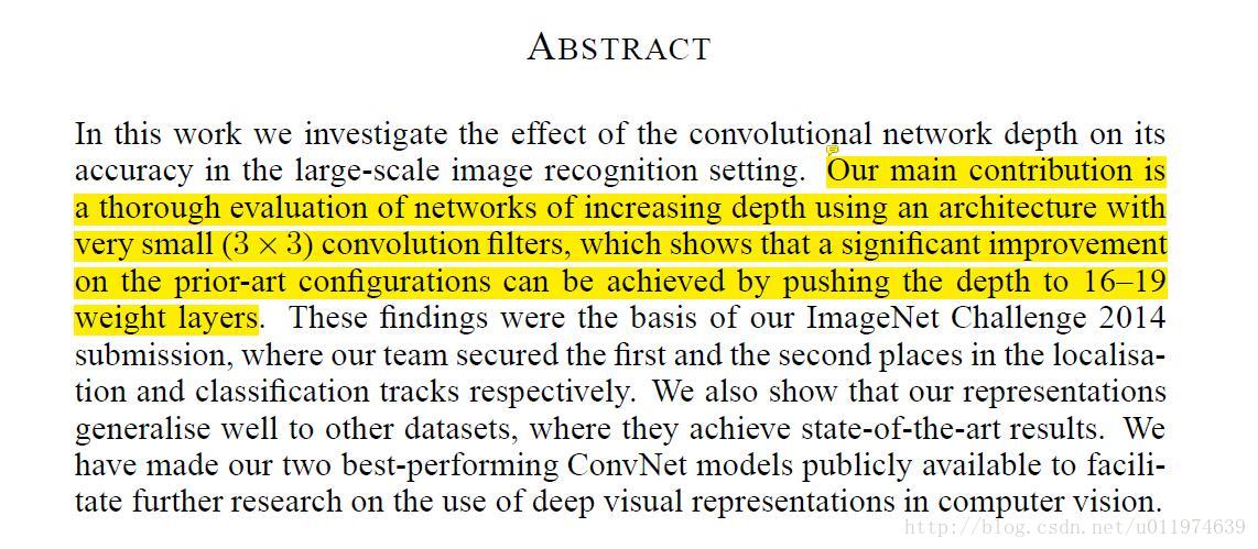
| Our main contribution is a thorough evaluation of networks of increasing depth using an architecture with very small (3×3) convolution filters, which shows that a significant improvement on the prior-art configurations can be achieved by pushing the depth to 16–19 weight layers. | 论文的主要研究方向: 主要评估小的卷积核(3*3)同等架构下随着网络深度的增加卷积网络的性能变化,随着网络深度到达16-19层,网络的性能也有着显著的提升。 |
1.介绍
| 原文 | description |
|---|---|
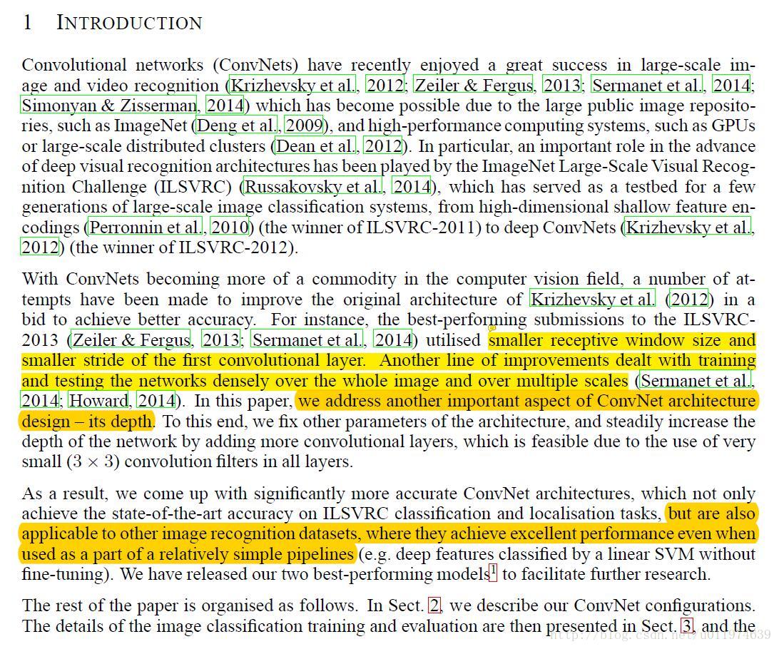
| utilised smaller receptive window size and smaller stride of the first convolutional layer. Another line of improvements dealt with training and testing the networks densely over the whole image and over multiple scales. we address another important aspect of ConvNet architecture design – its depth but are also applicable to other image recognition datasets, where they achieve excellent performance even when used as a part of a relatively simple pipelines |
当前卷积网络的研究方向和论文的关注点: 使用更小的感受野和在第一个卷积层上是有更短的步长,模型性能会更好(本文也是这个思想) 另一条提升模型性能的路线是使用多尺度的密集的训练和测试网络(论文后面探讨了Multi-crop和Multi-scale对模型性能的影响) 论文主要研究模型架构中叠加深度对性能的影响 vggnet在其他数据集上变现也非常好,迁移性很强 |
2.卷积网络配置
| 原文 | description |
|---|---|
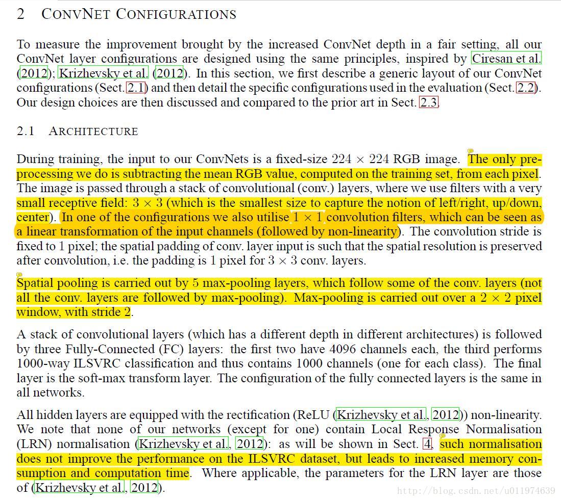
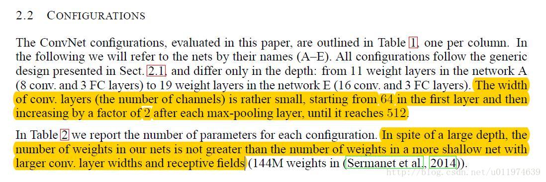
| The only preprocessing we do is subtracting the mean RGB value, computed on the training set, from each pixel small receptive field: 3 × 3 (which is the smallest size to capture the notion of left/right, up/down,center). In one of the configurations we also utilise 1 × 1 convolution filters, which can be seen as a linear transformation of the input channels (followed by non-linearity). Spatial pooling is carried out by 5 max-pooling layers, which follow some of the conv. layers (not all the conv. layers are followed by max-pooling). Max-pooling is carried out over a 2 × 2 pixel window, with stride 2. such normalisation does not improve the performance on the ILSVRC dataset, but leads to increased memory consumption and computation time |
VGGNet网络架构的设计: 数据集的预处理依旧是减去RGB均值(类似AlexNet中的处理) 使用更小的卷积核3*3(以为3*3刚好够捕获一个区域的信息) 使用1*1的卷积核,这是对输入做线性变换(当然输出经过了ReLU处理),这样的卷积核不改变输入通道的维度,并且可以提高模型的学习能力 网络的总体结构: 共有五个池化层,都是max-pooling层,每个最大池化层的池化核都是2*2,且步长都为2 论文认为AlexNet中使用的LRN层在ILSVRC数据集上没有提高性能,反倒是花费了大量的计算资源和计算时间。 |
| 原文 | description |
|---|---|
| The width of conv. layers (the number of channels) is rather small, starting from 64 in the first layer and then increasing by a factor of 2 after each max-pooling layer, until it reaches 512 In spite of a large depth, the number of weights in our nets is not greater than the number of weights in a more shallow net with larger conv. layer widths and receptive fields |
网络结构的配置: 因为使用的是小卷积核,使用的卷积核数目从64增加到512(每过一次max-pooling,卷积核数目x2倍) 是卷积层的卷积核的参数占总参数量的比例很少,但是对模型的性能影都很大 |
| 原文 | description |
|---|---|
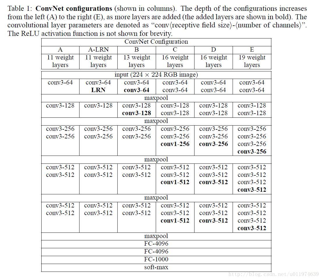
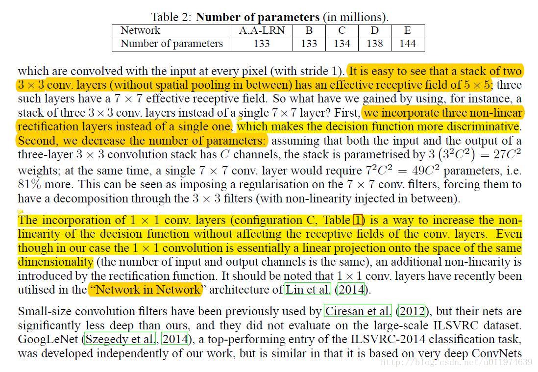
| It is easy to see that a stack of two 3×3 conv. layers (without spatial pooling in between) has an effective receptive field of 5×5; we incorporate three non-linear rectification layers instead of a single one, which makes the decision function more discriminative. Second, we decrease the number of parameters The incorporation of 1 × 1 conv. layers (configuration C, Table 1) is a way to increase the nonlinearity of the decision function without affecting the receptive fields of the conv. layers. Even though in our case the 1×1 convolution is essentially a linear projection onto the space of the same dimensionality |
网络结构中使用的技巧: 使用多个小卷积核堆叠,感受野与大卷积核相同.(后续有详解) 在多个小卷积核堆叠起来,会比单个大卷积核有更多激活函数的转换,学习能力会更强(多个ReLU处理) 并且,使用小卷积核会有着更少的参数 使用1*1的卷积核,可以增强决策函数的非线性,并且不会影响感受野, 即使在本论文模型使用1*1卷积核是同维度上的线性变换(1*1卷积后会经过ReLU处理,而ReLU在输入大于0是线性的) |
详解
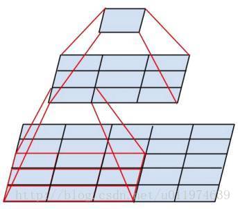
下图是两个3*3的卷积核堆叠在一起,可以看到:
- 在提取特征的能力上:
最顶层的1*1输出是由最底层的5*5的输入提取出来的,经过两个3*3的卷积核,效果与一个5*5的大卷积核类似。 - 在参数量上:
两个3*3的卷积核,有2*3*3=18参数,而一个5*5=25参数,可以看到参数量上也少了很多
分析网络参数量(这里以VGG16为例,论文中的D模型):
| 处理层 | shape | 占用显存 | 模型参数量 |
|---|---|---|---|
| INPUT | [224x224x3] | 224*224*3=150K | 0 |
| CONV3-64 | [224x224x64] | 224*224*64=3.2M | (3*3*3)*64 = 1,728=1.7K |
| CONV3-64 | [224x224x64] | 224*224*64=3.2M | (3*3*64)*64 = 36,864=37K |
| POOL2 | [112x112x64] | 112*112*64=800K | 0 |
| CONV3-128 | [112x112x128] | 112*112*128=1.6M | (3*3*64)*128 = 73,728=74K |
| CONV3-128 | [112x112x128] | 112*112*128=1.6M | (3*3*128)*128 = 147,456=147K |
| POOL2 | [56x56x128] | 56*56*128=400K | 0 |
| CONV3-256 | [56x56x256] | 56*56*256=800K | (3*3*128)*256 = 294,912=294K |
| CONV3-256 | [56x56x256] | 56*56*256=800K | (3*3*256)*256 = 589,824=590K |
| CONV3-256 | [56x56x256] | 56*56*256=800K | (3*3*256)*256 = 589,824=590K |
| POOL2 | [28x28x256] | 28*28*256=200K | 0 |
| CONV3-512 | [28x28x512] | 28*28*512=400K | (3*3*256)*512 = 1,179,648=1.2M |
| CONV3-512 | [28x28x512] | 28*28*512=400K | (3*3*512)*512 = 2,359,296=2.4M |
| CONV3-512 | [28x28x512] | 28*28*512=400K | (3*3*512)*512 = 2,359,296=2.4M |
| POOL2 | [14x14x512] | 14*14*512=100K | 0 |
| CONV3-512 | [14x14x512] | 14*14*512=100K | (3*3*512)*512 = 2,359,296=2.4M |
| CONV3-512 | [14x14x512] | 14*14*512=100K | (3*3*512)*512 = 2,359,296=2.4M |
| CONV3-512 | [14x14x512] | 14*14*512=100K | (3*3*512)*512 = 2,359,296=2.4M |
| POOL2 | [7x7x512] | 7*7*512=25K | 0 |
| FC | [1x1x4096] | 4096 | 7*7*512*4096 = 102,760,448=102.8M |
| FC | [1x1x4096] | 4096 | 4096*4096 = 16,777,216=16.8M |
| FC | [1x1x4096] | 1000 | 4096*1000 = 4,096,000=4M |
| 合计 | 24M*4bytes = 94MB/image (这只是一个前向传播) | 模型总的参数量:138M |
可以看到,大多数的显存消耗在前几个卷积层,而整个模型的大多数参数消耗在最后FC层。
3.分类框架
| 原文 | description |
|---|---|
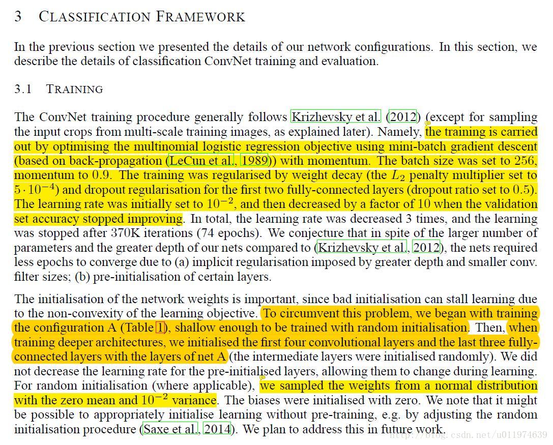
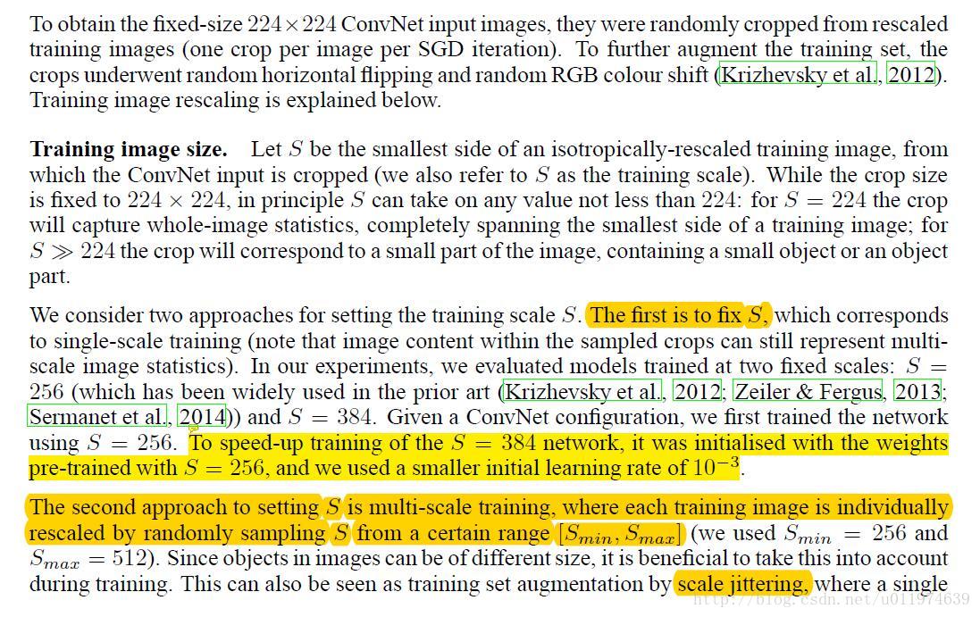
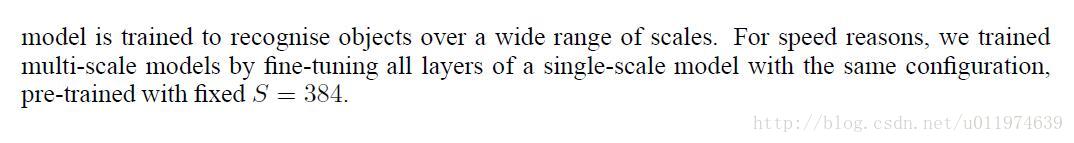
the training is carried out by optimising the multinomial logistic regression objective using mini-batch gradient descent (based on back-propagation (LeCun et al., 1989)) with momentum. The batch size was set to 256, momentum to 0.9. The training was regularised by weight decay (the L2 penalty multiplier set to 5 · 10−4) and dropout regularisation for the first two fully-connected layers (dropout ratio set to 0.5). The learning rate was initially set to 10−2, and then decreased by a factor of 10 when the validation set accuracy stopped improving. To circumvent this problem, we began with training the configuration A (Table 1), shallow enough to be trained with random initialisation. Then, when training deeper architectures, we initialised the first four convolutional layers and the last three fullyconnected layers with the layers of net A The first is to fix S,which corresponds to single-scale training . To speed-up training of the S = 384 network, it was initialised with the weights pre-trained with S = 256, and we used a smaller initial learning rate of 10−3 The second approach to setting S is multi-scale training, where each training image is individually rescaled by randomly sampling S from a certain range [Smin, Smax] |
训练上的处理: 和AlexNet类似,优化方式也是使用基于BP的mini-batch下的多logistic回归 模型的权值依旧是使用动量衰减的 FC层使用dropout技术;在学习率上也是初试到0.01,然后依旧在验证集上的表现,调整学习率(每当在验证集上错误率不变时,学习率下降10倍) 一个好的初始化权值是很重要的,为了解决这个问题,可以先训练一个深度较浅的网络A,再利于已经训练好的A网络权值初始化深度较深的网络。(迁移学习) 在数据集上处理,针对输入图片的尺寸上有两种方案: 第一种,使用固定的输入图片尺寸S,论文一共评估了两个S大小的模型,先是训练一个S=256的模型,再利用S=256的模型权值初始化一个尺寸S=384的模型权值,在训练S=384的模型; 第二种,使用变长的输入尺寸S,其中S是一个区间[Smin,Smax],下面还有对这两种训练方案的评估 |
| 原文 | description |
|---|---|
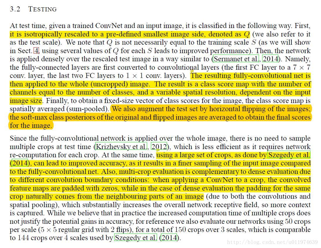
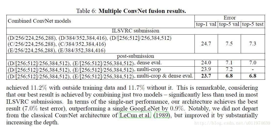
| We also augment the test set by horizontal flipping of the images; the soft-max class posteriors of the original and flipped images are averaged to obtain the final scores for the image using a large set of crops, as done by Szegedy et al. (2014), can lead to improved accuracy, as it results in a finer sampling of the input image compared to the fully-convolutional net. Also, multi-crop evaluation is complementary to dense evaluation due to different convolution boundary conditions: when applying a ConvNet to a crop, the convolved feature maps are padded with zeros, while in the case of dense evaluation the padding for the same crop naturally comes from the neighbouring parts of an image |
针对测试的处理: 对于测试的图片,使用水平翻转做图像增强,同时依旧是对多个输入在softmax层做平均输出 在做卷积操作时,边界填充的是0,而在multi-crop评估的情况下,填充的是来自图像的相邻部分 |
| 原文 | description |
|---|---|
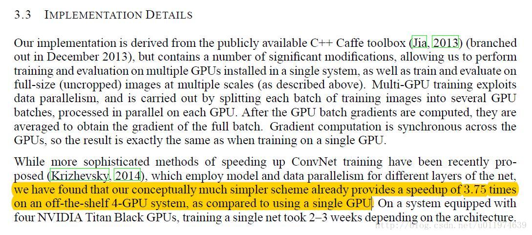
| we have found that our conceptuallymuch simpler scheme already provides a speedup of 3.75 times on an off-the-shelf 4-GPU system, as compared to using a single GPU. | 使用多GPU加速(现在的开源框架在计算资源集群上都做的很好了) |
4.分类实验
| 原文 | description |
|---|---|
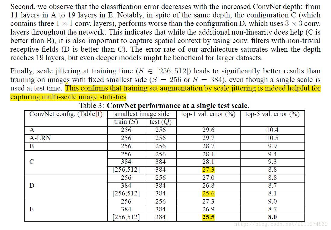
| This confirms that training set augmentation by scale jittering is indeed helpful for capturing multi-scale image statistics | 通过尺度抖动增强数据集有助于提升multi-scale的统计特性(模型性能更好) |
| 原文 | description |
|---|---|
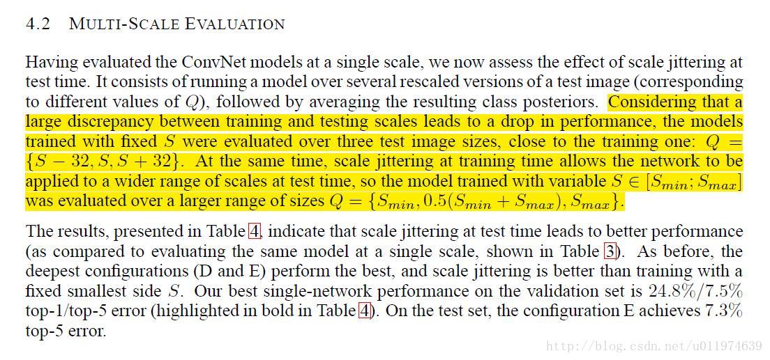
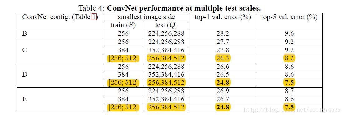
| Considering that a large discrepancy between training and testing scales leads to a drop in performance, the models trained with fixed S were evaluated over three test image sizes, close to the training one: Q = {S − 32, S, S + 32}. At the same time, scale jittering at training time allows the network to be applied to a wider range of scales at test time, so the model trained with variable S ∈ [Smin; Smax] was evaluated over a larger range of sizes Q = {Smin, 0.5(Smin + Smax), Smax}. |
考虑到由训练和测试的尺度不同导致性能上的巨大差异: 模型使用固定的训练输入尺寸S来评估三种尺寸的测试图片,即测试输入图片尺寸Q取{S-32,S,S+32}。 同时,我们可以对训练尺寸S做尺寸抖动,抖动范围为S ∈ [Smin; Smax],相对的测试图片的大小就变为 Q = {Smin, 0.5(Smin + Smax), Smax}. 在表格中,我们可以看见带尺寸抖动的模型是要优于不带抖动的 |
| 原文 | description |
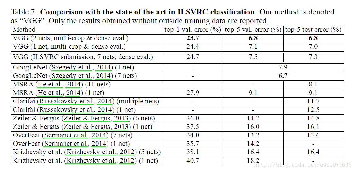
|---|---|
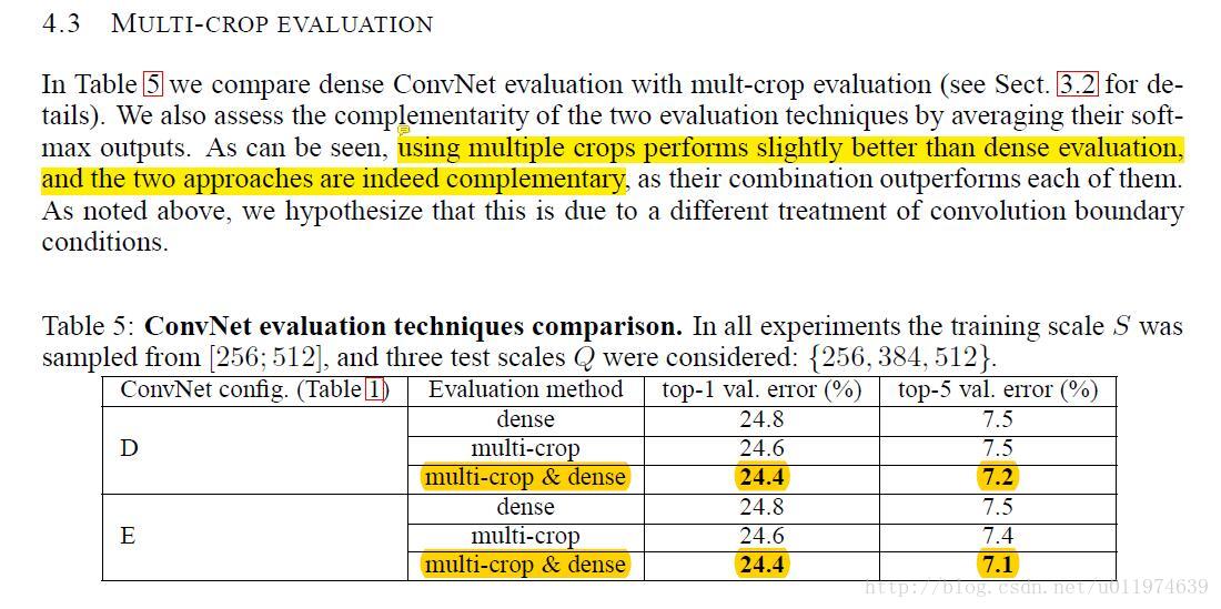
| using multiple crops performs slightly better than dense evaluation, and the two approaches are indeed complementary | multi-crop和dense evaluation 两种操作在对模型性能提升上是互补的 |
5.总结
VGGNet在TensorFlow里面实现
使用VGG16检测物体
VGGNet不像AlexNet那样容易训练,过深的层数在训练的过程中容易导致不收敛,从而模型爆炸,这里我们借用原论文的思想,使用pre-training,资料来自.toronto-Davi Frossard的博客。
文件介绍
一共包含四个文件:
- Model weights - vgg16_weights.npz
- TensorFlow model - vgg16.py
- Class names - imagenet_classes.py
- Example input - laska.png(我添加了其他文件,稍微修改了源代码)
介绍
在这篇短文中,我们提供了一个VGG16的实现以及从原来的Caffe模型转换成TensorFlow的权重。
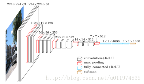
架构
VGG16的宏观架构如图1所示。 我们在文件vgg16.py中的TensorFlow中进行编码。 请注意,我们包括一个预处理层,其采用RGB图像,像素值范围为0-255,并减去平均图像值(在整个ImageNet训练集上计算)。
权重
我们使用专门的工具转换VGG作者在GitHub上公开的Caffe权重。 进行一些后期处理以确保模型与TensorFlow标准一致。 最后,我们得到vgg16_weights.npz中提供的权重。
代码介绍
# coding:utf8

########################################################################################
# Davi Frossard, 2016                                                                  #
# VGG16 implementation in TensorFlow                                                   #
# Details:                                                                             #
# http://www.cs.toronto.edu/~frossard/post/vgg16/                                      #
#                                                                                      #
# Model from https://gist.github.com/ksimonyan/211839e770f7b538e2d8#file-readme-md     #
# Weights from Caffe converted using https://github.com/ethereon/caffe-tensorflow


# update: 2017-7-30 delphifan
########################################################################################

import tensorflow as tf
import numpy as np
from scipy.misc import imread, imresize
from imagenet_classes import class_names


class vgg16:
    def __init__(self, imgs, weights=None, sess=None):
        self.imgs = imgs
        self.convlayers()
        self.fc_layers()
        self.probs = tf.nn.softmax(self.fc3l)  #计算softmax层输出
        if weights is not None and sess is not None:  #载入pre-training的权重
            self.load_weights(weights, sess)


    def convlayers(self):
        self.parameters = []

        # zero-mean input
        # 去RGB均值操作(这里RGB均值为原数据集的均值)
        with tf.name_scope('preprocess') as scope:
            mean = tf.constant([123.68, 116.779, 103.939],
                dtype=tf.float32, shape=[1, 1, 1, 3], name='img_mean')
            images = self.imgs-mean

        # conv1_1
        with tf.name_scope('conv1_1') as scope:
            kernel = tf.Variable(tf.truncated_normal([3, 3, 3, 64], dtype=tf.float32,
                                                     stddev=1e-1), name='weights')
            conv = tf.nn.conv2d(images, kernel, [1, 1, 1, 1], padding='SAME')
            biases = tf.Variable(tf.constant(0.0, shape=[64], dtype=tf.float32),
                                 trainable=True, name='biases')
            out = tf.nn.bias_add(conv, biases)
            self.conv1_1 = tf.nn.relu(out, name=scope)
            self.parameters += [kernel, biases]

        # conv1_2
        with tf.name_scope('conv1_2') as scope:
            kernel = tf.Variable(tf.truncated_normal([3, 3, 64, 64], dtype=tf.float32,
                                                     stddev=1e-1), name='weights')
            conv = tf.nn.conv2d(self.conv1_1, kernel, [1, 1, 1, 1], padding='SAME')
            biases = tf.Variable(tf.constant(0.0, shape=[64], dtype=tf.float32),
                                 trainable=True, name='biases')
            out = tf.nn.bias_add(conv, biases)
            self.conv1_2 = tf.nn.relu(out, name=scope)
            self.parameters += [kernel, biases]

        # pool1
        self.pool1 = tf.nn.max_pool(self.conv1_2,
                               ksize=[1, 2, 2, 1],
                               strides=[1, 2, 2, 1],
                               padding='SAME',
                               name='pool1')

        # conv2_1
        with tf.name_scope('conv2_1') as scope:
            kernel = tf.Variable(tf.truncated_normal([3, 3, 64, 128], dtype=tf.float32,
                                                     stddev=1e-1), name='weights')
            conv = tf.nn.conv2d(self.pool1, kernel, [1, 1, 1, 1], padding='SAME')
            biases = tf.Variable(tf.constant(0.0, shape=[128], dtype=tf.float32),
                                 trainable=True, name='biases')
            out = tf.nn.bias_add(conv, biases)
            self.conv2_1 = tf.nn.relu(out, name=scope)
            self.parameters += [kernel, biases]

        # conv2_2
        with tf.name_scope('conv2_2') as scope:
            kernel = tf.Variable(tf.truncated_normal([3, 3, 128, 128], dtype=tf.float32,
                                                     stddev=1e-1), name='weights')
            conv = tf.nn.conv2d(self.conv2_1, kernel, [1, 1, 1, 1], padding='SAME')
            biases = tf.Variable(tf.constant(0.0, shape=[128], dtype=tf.float32),
                                 trainable=True, name='biases')
            out = tf.nn.bias_add(conv, biases)
            self.conv2_2 = tf.nn.relu(out, name=scope)
            self.parameters += [kernel, biases]

        # pool2
        self.pool2 = tf.nn.max_pool(self.conv2_2,
                               ksize=[1, 2, 2, 1],
                               strides=[1, 2, 2, 1],
                               padding='SAME',
                               name='pool2')

        # conv3_1
        with tf.name_scope('conv3_1') as scope:
            kernel = tf.Variable(tf.truncated_normal([3, 3, 128, 256], dtype=tf.float32,
                                                     stddev=1e-1), name='weights')
            conv = tf.nn.conv2d(self.pool2, kernel, [1, 1, 1, 1], padding='SAME')
            biases = tf.Variable(tf.constant(0.0, shape=[256], dtype=tf.float32),
                                 trainable=True, name='biases')
            out = tf.nn.bias_add(conv, biases)
            self.conv3_1 = tf.nn.relu(out, name=scope)
            self.parameters += [kernel, biases]

        # conv3_2
        with tf.name_scope('conv3_2') as scope:
            kernel = tf.Variable(tf.truncated_normal([3, 3, 256, 256], dtype=tf.float32,
                                                     stddev=1e-1), name='weights')
            conv = tf.nn.conv2d(self.conv3_1, kernel, [1, 1, 1, 1], padding='SAME')
            biases = tf.Variable(tf.constant(0.0, shape=[256], dtype=tf.float32),
                                 trainable=True, name='biases')
            out = tf.nn.bias_add(conv, biases)
            self.conv3_2 = tf.nn.relu(out, name=scope)
            self.parameters += [kernel, biases]

        # conv3_3
        with tf.name_scope('conv3_3') as scope:
            kernel = tf.Variable(tf.truncated_normal([3, 3, 256, 256], dtype=tf.float32,
                                                     stddev=1e-1), name='weights')
            conv = tf.nn.conv2d(self.conv3_2, kernel, [1, 1, 1, 1], padding='SAME')
            biases = tf.Variable(tf.constant(0.0, shape=[256], dtype=tf.float32),
                                 trainable=True, name='biases')
            out = tf.nn.bias_add(conv, biases)
            self.conv3_3 = tf.nn.relu(out, name=scope)
            self.parameters += [kernel, biases]

        # pool3
        self.pool3 = tf.nn.max_pool(self.conv3_3,
                               ksize=[1, 2, 2, 1],
                               strides=[1, 2, 2, 1],
                               padding='SAME',
                               name='pool3')

        # conv4_1
        with tf.name_scope('conv4_1') as scope:
            kernel = tf.Variable(tf.truncated_normal([3, 3, 256, 512], dtype=tf.float32,
                                                     stddev=1e-1), name='weights')
            conv = tf.nn.conv2d(self.pool3, kernel, [1, 1, 1, 1], padding='SAME')
            biases = tf.Variable(tf.constant(0.0, shape=[512], dtype=tf.float32),
                                 trainable=True, name='biases')
            out = tf.nn.bias_add(conv, biases)
            self.conv4_1 = tf.nn.relu(out, name=scope)
            self.parameters += [kernel, biases]

        # conv4_2
        with tf.name_scope('conv4_2') as scope:
            kernel = tf.Variable(tf.truncated_normal([3, 3, 512, 512], dtype=tf.float32,
                                                     stddev=1e-1), name='weights')
            conv = tf.nn.conv2d(self.conv4_1, kernel, [1, 1, 1, 1], padding='SAME')
            biases = tf.Variable(tf.constant(0.0, shape=[512], dtype=tf.float32),
                                 trainable=True, name='biases')
            out = tf.nn.bias_add(conv, biases)
            self.conv4_2 = tf.nn.relu(out, name=scope)
            self.parameters += [kernel, biases]

        # conv4_3
        with tf.name_scope('conv4_3') as scope:
            kernel = tf.Variable(tf.truncated_normal([3, 3, 512, 512], dtype=tf.float32,
                                                     stddev=1e-1), name='weights')
            conv = tf.nn.conv2d(self.conv4_2, kernel, [1, 1, 1, 1], padding='SAME')
            biases = tf.Variable(tf.constant(0.0, shape=[512], dtype=tf.float32),
                                 trainable=True, name='biases')
            out = tf.nn.bias_add(conv, biases)
            self.conv4_3 = tf.nn.relu(out, name=scope)
            self.parameters += [kernel, biases]

        # pool4
        self.pool4 = tf.nn.max_pool(self.conv4_3,
                               ksize=[1, 2, 2, 1],
                               strides=[1, 2, 2, 1],
                               padding='SAME',
                               name='pool4')

        # conv5_1
        with tf.name_scope('conv5_1') as scope:
            kernel = tf.Variable(tf.truncated_normal([3, 3, 512, 512], dtype=tf.float32,
                                                     stddev=1e-1), name='weights')
            conv = tf.nn.conv2d(self.pool4, kernel, [1, 1, 1, 1], padding='SAME')
            biases = tf.Variable(tf.constant(0.0, shape=[512], dtype=tf.float32),
                                 trainable=True, name='biases')
            out = tf.nn.bias_add(conv, biases)
            self.conv5_1 = tf.nn.relu(out, name=scope)
            self.parameters += [kernel, biases]

        # conv5_2
        with tf.name_scope('conv5_2') as scope:
            kernel = tf.Variable(tf.truncated_normal([3, 3, 512, 512], dtype=tf.float32,
                                                     stddev=1e-1), name='weights')
            conv = tf.nn.conv2d(self.conv5_1, kernel, [1, 1, 1, 1], padding='SAME')
            biases = tf.Variable(tf.constant(0.0, shape=[512], dtype=tf.float32),
                                 trainable=True, name='biases')
            out = tf.nn.bias_add(conv, biases)
            self.conv5_2 = tf.nn.relu(out, name=scope)
            self.parameters += [kernel, biases]

        # conv5_3
        with tf.name_scope('conv5_3') as scope:
            kernel = tf.Variable(tf.truncated_normal([3, 3, 512, 512], dtype=tf.float32,
                                                     stddev=1e-1), name='weights')
            conv = tf.nn.conv2d(self.conv5_2, kernel, [1, 1, 1, 1], padding='SAME')
            biases = tf.Variable(tf.constant(0.0, shape=[512], dtype=tf.float32),
                                 trainable=True, name='biases')
            out = tf.nn.bias_add(conv, biases)
            self.conv5_3 = tf.nn.relu(out, name=scope)
            self.parameters += [kernel, biases]

        # pool5
        self.pool5 = tf.nn.max_pool(self.conv5_3,
                               ksize=[1, 2, 2, 1],
                               strides=[1, 2, 2, 1],
                               padding='SAME',
                               name='pool4')

    def fc_layers(self):
        # fc1
        with tf.name_scope('fc1') as scope:
             # 取出shape中第一个元素后的元素  例如x=[1,2,3] -->x[1:]=[2,3]
             # np.prod是计算数组的元素乘积 x=[2,3] np.prod(x) = 2*3 = 6
             # 这里代码可以使用 shape = self.pool5.get_shape()
             #shape = shape[1].value * shape[2].value * shape[3].value 代替
            shape = int(np.prod(self.pool5.get_shape()[1:]))
            fc1w = tf.Variable(tf.truncated_normal([shape, 4096],
                                                         dtype=tf.float32,
                                                         stddev=1e-1), name='weights')
            fc1b = tf.Variable(tf.constant(1.0, shape=[4096], dtype=tf.float32),
                                 trainable=True, name='biases')
            pool5_flat = tf.reshape(self.pool5, [-1, shape])
            fc1l = tf.nn.bias_add(tf.matmul(pool5_flat, fc1w), fc1b)
            self.fc1 = tf.nn.relu(fc1l)
            self.parameters += [fc1w, fc1b]

        # fc2
        with tf.name_scope('fc2') as scope:
            fc2w = tf.Variable(tf.truncated_normal([4096, 4096],
                                                         dtype=tf.float32,
                                                         stddev=1e-1), name='weights')
            fc2b = tf.Variable(tf.constant(1.0, shape=[4096], dtype=tf.float32),
                                 trainable=True, name='biases')
            fc2l = tf.nn.bias_add(tf.matmul(self.fc1, fc2w), fc2b)
            self.fc2 = tf.nn.relu(fc2l)
            self.parameters += [fc2w, fc2b]

        # fc3
        with tf.name_scope('fc3') as scope:
            fc3w = tf.Variable(tf.truncated_normal([4096, 1000],
                                                         dtype=tf.float32,
                                                         stddev=1e-1), name='weights')
            fc3b = tf.Variable(tf.constant(1.0, shape=[1000], dtype=tf.float32),
                                 trainable=True, name='biases')
            self.fc3l = tf.nn.bias_add(tf.matmul(self.fc2, fc3w), fc3b)
            self.parameters += [fc3w, fc3b]

    def load_weights(self, weight_file, sess):
        weights = np.load(weight_file)
        keys = sorted(weights.keys())
        for i, k in enumerate(keys):
            print i, k, np.shape(weights[k])
            sess.run(self.parameters[i].assign(weights[k]))

if __name__ == '__main__':
    sess = tf.Session()
    imgs = tf.placeholder(tf.float32, [None, 224, 224, 3])
    vgg = vgg16(imgs, 'vgg16_weights.npz', sess)  # 载入预训练好的模型权重

    img1 = imread('images.jpg', mode='RGB')    #载入需要判别的图片
    img1 = imresize(img1, (224, 224))

    img2 = imread('dog.jpg', mode='RGB')
    img2 = imresize(img2, (224, 224))

    img3 = imread('laska.png', mode='RGB')
    img3 = imresize(img3, (224, 224))

    #计算VGG16的softmax层输出(返回是列表,每个元素代表一个判别类型的数组)
    prob = sess.run(vgg.probs, feed_dict={vgg.imgs: [img1, img2, img3]})

    for pro in prob:
        # 源代码使用(np.argsort(prob)[::-1])[0:5]
        # np.argsort(x)返回的数组值从小到大的索引值
        #argsort(-x)从大到小排序返回索引值   [::-1]是使用切片将数组从大到小排序
        #preds = (np.argsort(prob)[::-1])[0:5]
        preds = (np.argsort(-pro))[0:5]  #取出top5的索引
        for p in preds:
            print class_names[p], pro[p]
        print '\n'
- 1
- 2
- 3
- 4
- 5
- 6
- 7
- 8
- 9
- 10
- 11
- 12
- 13
- 14
- 15
- 16
- 17
- 18
- 19
- 20
- 21
- 22
- 23
- 24
- 25
- 26
- 27
- 28
- 29
- 30
- 31
- 32
- 33
- 34
- 35
- 36
- 37
- 38
- 39
- 40
- 41
- 42
- 43
- 44
- 45
- 46
- 47
- 48
- 49
- 50
- 51
- 52
- 53
- 54
- 55
- 56
- 57
- 58
- 59
- 60
- 61
- 62
- 63
- 64
- 65
- 66
- 67
- 68
- 69
- 70
- 71
- 72
- 73
- 74
- 75
- 76
- 77
- 78
- 79
- 80
- 81
- 82
- 83
- 84
- 85
- 86
- 87
- 88
- 89
- 90
- 91
- 92
- 93
- 94
- 95
- 96
- 97
- 98
- 99
- 100
- 101
- 102
- 103
- 104
- 105
- 106
- 107
- 108
- 109
- 110
- 111
- 112
- 113
- 114
- 115
- 116
- 117
- 118
- 119
- 120
- 121
- 122
- 123
- 124
- 125
- 126
- 127
- 128
- 129
- 130
- 131
- 132
- 133
- 134
- 135
- 136
- 137
- 138
- 139
- 140
- 141
- 142
- 143
- 144
- 145
- 146
- 147
- 148
- 149
- 150
- 151
- 152
- 153
- 154
- 155
- 156
- 157
- 158
- 159
- 160
- 161
- 162
- 163
- 164
- 165
- 166
- 167
- 168
- 169
- 170
- 171
- 172
- 173
- 174
- 175
- 176
- 177
- 178
- 179
- 180
- 181
- 182
- 183
- 184
- 185
- 186
- 187
- 188
- 189
- 190
- 191
- 192
- 193
- 194
- 195
- 196
- 197
- 198
- 199
- 200
- 201
- 202
- 203
- 204
- 205
- 206
- 207
- 208
- 209
- 210
- 211
- 212
- 213
- 214
- 215
- 216
- 217
- 218
- 219
- 220
- 221
- 222
- 223
- 224
- 225
- 226
- 227
- 228
- 229
- 230
- 231
- 232
- 233
- 234
- 235
- 236
- 237
- 238
- 239
- 240
- 241
- 242
- 243
- 244
- 245
- 246
- 247
- 248
- 249
- 250
- 251
- 252
- 253
- 254
- 255
- 256
- 257
- 258
- 259
- 260
- 261
- 262
- 263
- 264
- 265
- 266
- 267
- 268
- 269
- 270
- 271
- 272
- 273
- 274
- 275
- 276
- 277
- 278
- 279
- 280
- 281
- 282
- 283
- 284
- 285
- 286
- 287
- 288
- 289
- 290
- 291
- 292
- 293
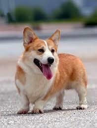
这里面使用的测试图images.jpg和dog.jpg如下:
images.jpg
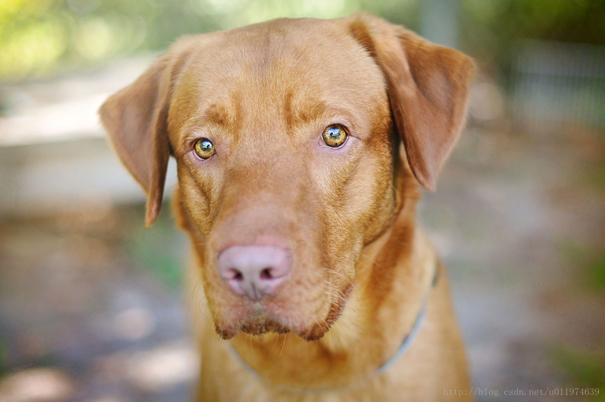
dog.jpg
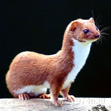
laska.png
测试输出:
Pembroke, Pembroke Welsh corgi 0.934712 #柯基
Cardigan, Cardigan Welsh corgi 0.0646527
dingo, warrigal, warragal, Canis dingo 0.000343477
Chihuahua 7.22381e-05
Eskimo dog, husky 4.01941e-05
vizsla, Hungarian pointer 0.723731 #匈牙利猎犬
Rhodesian ridgeback 0.271104
Chesapeake Bay retriever 0.00191715
Labrador retriever 0.00120256
redbone 0.000673155
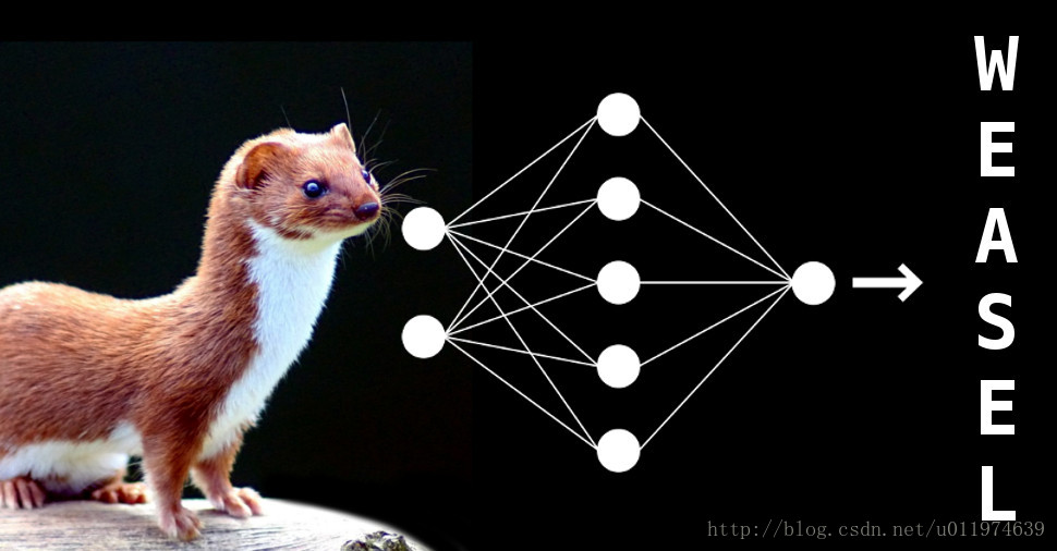
weasel 0.693388 #黄鼠狼
polecat, fitch, foulmart, foumart, Mustela putorius 0.175386
mink 0.122086
black-footed ferret, ferret, Mustela nigripes 0.00887065
otter 0.000121083
- 1
- 2
- 3
- 4
- 5
- 6
- 7
- 8
- 9
- 10
- 11
- 12
- 13
- 14
- 15
- 16
- 17
- 18
- 19
- 20
效果还是非常好的!有兴趣的可以试试其他图片
总结
VGGNet相比AlexNet进步非常大,在AlexNet的基础上,研究了小卷积核下堆叠卷积层对模型的性能影响,其中提出的pre-training技术被广泛使用(迁移学习)。VGGNet的模型参数虽然比AlexNet多,但反而只需要较少的迭代次数就可以收敛,凭借其相对不算很高的复杂度和优秀的分类性能,称为一代经典的卷积神经网络,直到现在依然被应用在很多地方。
到这里算是介绍完AlexNet和VGGNet,后续继续介绍其他经典的CNN模型~
参考资料
《TensorFlow实战》 -黄文坚等
Stanford University CS231n学习课程 http://cs231n.stanford.edu/
https://www.cs.toronto.edu/~frossard/post/vgg16/
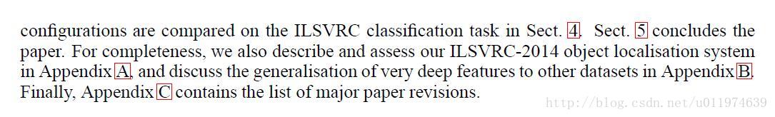
引言
上一章节,我们学习了CNN模型的发展历史和应用领域,同时细致的剖析了模型的结构和原理,也简单的学习了在TensorFlow内有关CNN的api。最后在MNIST和CIFAR10数据集上验证了CNN模型强大的特征提取能力。
本章节将学习经典的CNN模型,这几个CNN模型都曾在ImageNet大赛上大放光彩,也代表着这几年CNN模型的发展路线。
本节重点放在AlexNet和VGGNet上,下面表格是两个网络的简单比较:
| 特点 | AlexNet | VGGNet |
|---|---|---|
| 论文贡献 | 介绍完整CNN架构模型(近些年的许多CNN模型都是依据此模型变种来的)和多种训练技巧 CNN模型复兴的开山之作 使用GPU加速训练,让CNN模型训练得以实现 |
讨论了在小卷积核下,模型性能随着堆叠层数加深的变化 同时探讨multi-crop和dense evaluation对模型性能的影响 |
| 网络结构 | 1.AlexNet的网络架构成为了大型CNN模型的经典架构 2.成功的使用了ReLU激活函数 3.成功的应用了(重叠)最大池化层 |
1.多个小卷积核层堆叠(模型的迁移性能较好) 2.使用1*1卷积核增强模型的判别能力 |
| 训练Tricks | 1.数据增强,包括对训练数据做取RGB均值,随机截取固定尺寸,做水平翻转扩大训练集; 2.使用dropout技术增强模型的鲁棒性和泛化能力 3.测试时,对测试图片做数据增强,同时在softmax层去均值再输出 4.带动量的权值衰减 5.学习率在验证集上的错误率不提高时下降10倍 |
训练简单模型A,使用模型A的权值初始化复杂模型B(迁移学习) 数据增强,对训练数据去RGB均值,做水平翻转扩大训练集; 使用dropout技术 测试时,对测试图片做数据增强,在softmax层 带动量的权值衰减 学习率在验证集上的错误率不提高时下降10倍 |
| 其他观点 | LRN层有助于增强模型泛化能力 | LRN效果甚微,反倒的计算量增加不少 |
AlexNet
AlexNet 简介
2012年,Hinton的学生Alex提出了CNN模型AlexNet,AlexNet可以算是LeNet的一种更深更宽的版本。同年AlexNet以显著优势获得了IamgeNet的冠军,top-5错误率降低到了16.4%,相比于第二名26.2%的错误路有了巨大的提升,而AlexNet模型的参数量还不到第二名模型的二分之一。AlexNet可以说是神经网络在低谷期后第一次发威,确立了深度学习在计算机视觉领域的统治地位,同时也推动了深度学习在语音识别、自然语言处理、强化学习等领域的拓展。
AlexNet的特点
- 针对网络架构:
- 成功的使用ReLU作为激活函数,并验证其效果在较深的网络要优于Sigmoid.
- 使用LRN层,对局部神经元的活动创建竞争机制,使得其中响应比较大的值变的相对更大,并抑制其他反馈较小的神经元,增强了模型的泛化能力。
- 使用重叠的最大池化,论文中提出让步长比池化核的尺寸小,这样池化层的输出之间会有重叠和覆盖,提升了特征的丰富性。
- 针对过拟合现象:
- 数据增强,对原始图像随机的截取输入图片尺寸大小(以及对图像作水平翻转操作),使用数据增强后大大减轻过拟合,提升模型的泛化能力。同时,论文中会对原始数据图片的RGB做PCA分析,并对主成分做一个标准差为0.1的高斯扰动。
- 使用Dropout随机忽略一部分神经元,避免模型过拟合。
- 针对训练速度:
- 使用GPU计算,加快计算速度
AlexNet论文分析
引言
| 原文 | description |
|---|---|
| The neural network, which has 60 million parameters and 650,000 neurons, consists of five convolutional layers, some of which are followed by max-pooling layers,and three fully-connected layers with a final 1000-way softmax. |
介绍了AlexNet网络结构: 五个卷积层(若干卷积层包含最大池化层)三个全连接层(最后一层为1000分类的softmax) 超过六千万参数和六十五万神经元 |
| To reduce overfitting in the fully-connected layers we employed a recently-developed regularization method called “dropout” that proved to be very effective. | 减少全连接层的过拟合情况: 使用dropout方法防治overfitting (后续有详解) |
1. 介绍
| 原文 | description |
|---|---|
| datasets of labeled images were relatively small… especially if they are augmented with label-preserving transformations… But objects in realistic settings exhibit considerable variability… |
指出传统数据集和模型存在的问题: 数据集较小时,通过数据增强等技术,模型可在简单的识别任务上表现很好 但是在现实复杂环境识别任务上表现的不尽人意 进而引出了ImageNet数据集 |
| so our model should also have lots of prior knowledge Their capacity can be controlled by varying their depth and breadth and they also make strong and mostly correct assumptions about the nature of images CNNs have much fewer connections and parameters and so they are easier to train, while their theoretically-best performance is likely to be only slightly worse. |
点出为什么用CNN模型,CNN模型的优点? 我们的模型需要足够的先验知识 CNN的性能可以通过扩展宽度和深度来控制 CNN的参数相对来说较少,从而可训练 CNN的表现可观 |
| 原文 | description |
|---|---|
| current GPUs The size of our network made overfitting a significant problem we found that removing any convolutional layer resulted in inferior performance. our results can be improved simply by waiting for faster GPUs and bigger datasets to become available. |
CNN模型优缺点: 因为GPU,现在可以实现CNN模型的训练 这样多参数的模型,过拟合现象依旧是一个大问题 模型的深度看起来看重要,移除任何一个卷积层,模型的性能都会大大降低 提升模型性能简单的方法是使用更好的GPU和更大的数据集 |
2. 数据集
| 原文 | description |
|---|---|
| we down-sampled the images to a fixed resolution of 256 x 256. except for subtracting the mean activity over the training set from each pixel. |
数据集的处理方式: 对图片做放缩,下采样得到标准矩形大小为256x256图像 输入图像做去均值操作(后续有详解) |
3. 网络架构
| 原文 | description |
|---|---|
| In terms of training time with gradient descent, these saturating nonlinearities are much slower than the non-saturating nonlinearity f(x) = max(0, x). but networks with ReLUs consistently learn several times faster than equivalents with saturating neurons. on this dataset the primary concern is preventing overfitting |
ReLU激活函数的应用: 传统的激活函数,例如sigmoid或tanh会存在梯度弥散/消失问题,导致训练速度降低 以前的paper使用ReLU配置均值池化来防止过拟合,本文使用ReLU激活函数可以大幅度提高训练速度 |
注解
如图可以看到sigmoid、tanh函数存在饱和区,即在输入取较大或者较小值时,输出值饱和。这样的激活函数存在一个问题:在饱和区域,gradient较小,尤其是在深度网络中,会有gradient vanishing的问题,导致训练收敛速度降低。
ReLU函数的特性决定了在大部分情况下,其gradient为常数,有利于BP的误差传递。
同时还有一个特性(个人见解):ReLU函数当输入小于等于零,输出也为零,这和dropout技术(下面有解释)有点相似,可以提高模型的鲁棒性。
当然,这里不是说ReLU就一定比sigmoid或tanh好,ReLU的不是全程可导(优势:ReLU的导数计算比sigmoid或tanh简单的多);ReLU的输出范围区间不可控。
现在GPU单卡的计算力和显存可以放下整个AlexNet了,这里就不过分讨论论文里关于使用多GPU加速计算的内容了
| 原文 | description |
|---|---|
| we still find that the following local normalization scheme aids generalization. This sort of response normalization implements a form of lateral inhibition inspired by the type found in real neurons, creating competition for big activities amongst neuron outputs computed using different kernels. Response normalization reduces our top-1 and top-5 error rates by 1.4% and 1.2%, respectively. |
论文有关于局部响应归一化的看法: 在ReLU后,做LRN处理可以提高模型的泛化能力 LRN处理类似于生物神经元的横向抑制机制,可以理解为将局部响应最大的再放大,并抑制其他响应较小的(我的理解这是放大局部显著特征,作用还是提高鲁棒性) 在AlexNet中加LRN层可以降低错误率(在下一篇VGGNet论文中实验指出LRN并不能降低错误率,反倒加大了计算量,LRN的应用场合还需要再考量) |
| 原文 | description |
|---|---|
| each summarizing a neighborhood of size z * z centered at the location of the pooling unit. If we set s < z, we obtain overlapping pooling We generally observe during training that models with overlapping pooling find it slightly more difficult to overfit. |
重叠最大池化层的使用: 池化核的大小为z * z,如果移动的步长s < z,就得到了重叠的池化结果 使用重叠的池化层可以增强模型提取特征的能力,有利于防止过拟合 |
| 原文 | description |
|---|---|
| Our network maximizes the multinomial logistic regression objective, which is equivalent to maximizing the average across training cases of the log-probability of the correct label under the prediction distribution. The neurons in the fully connected layers are connected to all neurons in the previous layer. Response-normalization layers follow the first and second convolutional layers. Max-pooling layers follow both response-normalization layers as well as the fifth convolutional layer. The ReLU non-linearity is applied to the output of every convolutional and fully-connected layer. The third, fourth, and fifth convolutional layers are connected to one another without any intervening pooling or normalization layers. |
详解介绍的一下网络架构: 网络最大化了多项logistic回归目标,等同于在预测分布下最大化了训练样本中正确标签的对数概率的平均值(softmax定义) FC层与上一层是全连接的,包括第五层卷积层输出与FC一层也是全连接的;第一层卷积和第二层卷积后有LRN层,再跟最大池化层 每一个卷积层后都做ReLU处理,第一第二卷积层后的LRN层也是处理ReLU的输出 第三层/第四层和第五层卷积层只单单做卷积,没有池化或LRN层 |
注解
(下面使用的结构与AlexNet类似,不全相同(AlexNet分GPU训练,连接方式不同))
AlexNet的网络计算流程如下图:
| 连接层 | 计算流程 |
|---|---|
| 第一卷积层 | 输入–>卷积–>ReLUs–>LRN–>max-pooling |
| 第二卷积层 | 卷积–>ReLUs–>LRN–>max-pooling |
| 第三卷积层 | 卷积–>ReLUs |
| 第四卷积层 | 卷积–>ReLUs |
| 第五卷积层 | 卷积–>ReLUs |
| 第一全连接层 | 矩阵乘法–>ReLUs–>dropout(后面会介绍) |
| 第二全连接层 | 矩阵乘法–>ReLUs–>dropout |
| 第三全连接层(softmax层) | 矩阵乘法–>ReLUs–>softmax |
整体的计算架构(简化了ReLU、LRN、Dropout等操作)如下:
| 操作层 | 结果 | 操作步骤 |
|---|---|---|
| INPUT | [227x227x3] | 注:论文标准是224(实际计算应该是227) |
| CONV1 | [55x55x96] | 96 11x11 filters at stride 4, pad 0 (227-11)/4 + 1 = 55 |
| MAX POOL1 | [27x27x96] | 3x3 filters at stride 2 (55-3)/2 + 1 = 27 |
| CONV2 | [27x27x256] | 256 5x5 filters at stride 1, pad 2 (27-5 + 2*2)/1 + 1 = 27 |
| MAX POOL2 | [13x13x256] | 3x3 filters at stride 2 (27 -3)/2 + 1 = 13 |
| CONV3 | [13x13x384] | 384 3x3 filters at stride 1, pad 1 (13-3 + 2*1)/1 + 1 = 13 |
| CONV4 | [13x13x384] | 384 3x3 filters at stride 1, pad 1 (13-3 + 2*1)/1 + 1 = 13 |
| CONV5 | [13x13x256] | 256 3x3 filters at stride 1, pad 1 (13-3 + 2*1)/1 + 1 = 13 |
| MAX POOL3 | [6x6x256] | 3x3 filters at stride 2 (13-3)/2 + 1 = 6 |
| FC1 | [4096] | 4096 neurons |
| FC2 | [4096] | 4096 neurons |
| SOFTMAX | [1000] | 1000 neurons |
模型使用的资源如下:
| 连接层 | 参数量 | 占用显存量(GPU训练一张图片) |
|---|---|---|
| 第一卷积层 | 34K | 500K |
| 第二卷积层 | 600K | 220K |
| 第三卷积层 | 860K | 60K |
| 第四卷积层 | 1300K | 60K |
| 第五卷积层 | 870K | 49K |
| 第一全连接层 | 36870K | 4K |
| 第二全连接层 | 16380K | 4K |
| 第三全连接层(softmax层) | 4000K | 1K |
| 合计 | 一张图片:60M*4bytes = 240M | 900K |
4. 减少过拟合
| 原文 | description |
|---|---|
| The first form of data augmentation consists of generating image translations and horizontal reflections. This increases the size of our training set by a factor of 2048, though the resulting training examples are, of course, highly interdependent. At test time, the network makes a prediction by extracting five 224 * 224 patches (the four corner patches and the center patch) as well as their horizontal reflections (hence ten patches in all), and averaging the predictions made by the network’s softmax layer on the ten patches. The second form of data augmentation consists of altering the intensities of the RGB channels in training images. Specifically, we perform PCA on the set of RGB pixel values throughout the ImageNet training set. To each training image, we add multiples of the found principal components,with magnitudes proportional to the corresponding eigenvalues times a random variable drawn from a Gaussian with mean zero and standard deviation 0.1. This scheme approximately captures an important property of natural images, namely, that object identity is invariant to changes in the intensity and color of the illumination. |
有关于减少过拟合现象的操作: 第一种方式:数据增强 通过随机截取输入中固定大小的图片,并做水平翻转,扩大数据集,减少过拟合情况 数据集可扩大到原来的2048倍 (256-224)^2 * 2 = 2048 在做预测时,取出测试图片的十张patch(四角+中间,再翻转)作为输入,十张patch在softmax层输出相加去平均值作为最后的输出结果 第二种方式:改变训练图片的RGB通道值 对原训练集做PCA(主成分分析),对每一张训练图片,加上多倍的主成分 (个人理解:这样操作类似于信号处理中的去均值,消除直流分量的影响) 经过做PCA分析的处理,减少了模型的过拟合现象。可以得到一个自然图像的性质,改变图像的光照的颜色和强度,目标的特性是不变的,并且这样的处理有利于减少过拟合。 |
| 原文 | description |
|---|---|
| a very efficient version of model combination that only costs about a factor of two during training. The recently-introduced technique, called “dropout” [10], consists of setting to zero the output of each hidden neuron with probability 0.5. every time an input is presented, the neural network samples a different architecture, but all these architectures share weights. This technique reduces complex co-adaptations of neurons, since a neuron cannot rely on the presence of particular other neurons. It is, therefore, forced to learn more robust features that are useful in conjunction with many different random subsets of the other neurons. we use all the neurons but multiply their outputs by 0.5, which is a reasonable approximation to taking the geometric mean of the predictive distributions produced by the exponentially-many dropout networks. |
使用dropout减少过拟合现象: dropout技术即让hidden层的神经元以50%的概率参与前向传播和反向传播. dropout技术减少了神经元之间的耦合,在每一次传播的过程中,hidden层的参与传播的神经元不同,整个模型的网络就不相同了,这样就会强迫网络学习更robust的特征,从而提高了模型的鲁棒性 对采用dropout技术的层,在输出时候要乘以0.5,这是一个合理的预测分布下的几何平均数的近似 |
5. 训练细节
| 原文 | description |
|---|---|
| We found that this small amount of weight decay was important for the model to learn. In other words, weight decay here is not merely a regularizer: it reduces the model’s training error. We initialized the neuron biases in the second, fourth, and fifth convolutional layers, as well as in the fully-connected hidden layers, with the constant 1. This initialization accelerates the early stages of learning by providing the ReLUs with positive inputs. We initialized the neuron biases in the remaining layers with the constant 0. The heuristic which we followed was to divide the learning rate by 10 when the validation error rate stopped improving with the current learning rate |
在训练调试上的细节描述: 使用小幅度的权值衰减,很利于模型的训练学习 对于第二、第四、第五卷积层还有全连接层,我们将bias初始化为1,有利于给ReLU提供一个正输入,加快训练速度 ;剩下的层bias初始化为0 学习率我们初始化为0.01,当模型在验证集错误率不提升时,我们将学习率降低10倍,整个训练过程降低了三次 |
6. 结果
| 原文 | description |
|---|---|
| The remaining columns show the six training images that produce feature vectors in the last hidden layer with the smallest Euclidean distance from the feature vector for the test image. If two images produce feature activation vectors with a small Euclidean separation, we can say that the higher levels of the neural network consider them to be similar. |
模型结果的分析: 图片右边展示了和测试图片在输出层上向量欧式距离很小的几张图片,可以看到这几张图片非常相似 我们可以得出结论,在特征激活向量的欧式距离相差较小的话,可以认为两张图片非常相似 |
7. 讨论
参考文献(略…)
AlexNet在TensorFlow里面实现
TensorFlow官方给出的AlexNet实现
首先给出的是TensorFlow官方的AlexNet实现,因为ImageNet数据集太大,所以官方是代码实现计算了前向和反向的训练时间,并没有真正的训练模型。其后,我在MNIST和CIFAR10上测试了AlexNet的性能。
实现代码
源代码在
models.tutorials.image.alexnet.alexnet_benchmark.py
- 1
实际代码如下:
# coding:utf8
# Copyright 2015 The TensorFlow Authors. All Rights Reserved.
#
# Licensed under the Apache License, Version 2.0 (the "License");
# you may not use this file except in compliance with the License.
# You may obtain a copy of the License at
#
#     http://www.apache.org/licenses/LICENSE-2.0
#
# Unless required by applicable law or agreed to in writing, software
# distributed under the License is distributed on an "AS IS" BASIS,
# WITHOUT WARRANTIES OR CONDITIONS OF ANY KIND, either express or implied.
# See the License for the specific language governing permissions and
# limitations under the License.
# ==============================================================================


"""Timing benchmark for AlexNet inference.

To run, use:
  bazel run -c opt --config=cuda \
      models/tutorials/image/alexnet:alexnet_benchmark

Across 100 steps on batch size = 128.

Forward pass:
Run on Tesla K40c: 145 +/- 1.5 ms / batch
Run on Titan X:     70 +/- 0.1 ms / batch

Forward-backward pass:
Run on Tesla K40c: 480 +/- 48 ms / batch
Run on Titan X:    244 +/- 30 ms / batch
"""
from __future__ import absolute_import
from __future__ import division
from __future__ import print_function

import argparse
from datetime import datetime
import math
import sys
import time

from six.moves import xrange  # pylint: disable=redefined-builtin
import tensorflow as tf

FLAGS = None


def print_activations(t):
  '''
    展示一个Tensor的name和shape
  :param t:
  :return:
  '''
  print(t.op.name, ' ', t.get_shape().as_list())


def inference(images):
  '''
   定义了AlexNet的前五个卷积层(FC计算速度较快,这里不做考虑)
  :param images: 输入图像Tensor
  :return:  返回最后一层pool5和parameters
  '''
  parameters = []

  # conv1
  # 使用name_scope可以将scope内创建的Variable命名conv1/xxx,便于区分不同卷积层的参数
  # 64个卷积核为11*11*3,步长为4,初始化权值为截断的正态分布(标注差为0.1)
  with tf.name_scope('conv1') as scope:
    kernel = tf.Variable(tf.truncated_normal([11, 11, 3, 64], dtype=tf.float32,
                                             stddev=1e-1), name='weights')
    conv = tf.nn.conv2d(images, kernel, [1, 4, 4, 1], padding='SAME')
    biases = tf.Variable(tf.constant(0.0, shape=[64], dtype=tf.float32),
                         trainable=True, name='biases')
    bias = tf.nn.bias_add(conv, biases)
    conv1 = tf.nn.relu(bias, name=scope)
    print_activations(conv1)
    parameters += [kernel, biases]

  # lrn1
  #
  with tf.name_scope('lrn1') as scope:
    lrn1 = tf.nn.lrn(conv1, alpha=1e-4, beta=0.75, depth_radius=2, bias=2.0)

  # pool1
  # 池化核3*3 步长为2*2
  pool1 = tf.nn.max_pool(lrn1, ksize=[1, 3, 3, 1], strides=[1, 2, 2, 1], padding='VALID')
  print_activations(pool1)

  # conv2
  # 192个卷积核为5*5*64,步长为1,初始化权值为截断的正态分布(标注差为0.1)
  with tf.name_scope('conv2') as scope:
    kernel = tf.Variable(tf.truncated_normal([5, 5, 64, 192], dtype=tf.float32,
                                             stddev=1e-1), name='weights')
    conv = tf.nn.conv2d(pool1, kernel, [1, 1, 1, 1], padding='SAME')
    biases = tf.Variable(tf.constant(0.0, shape=[192], dtype=tf.float32),
                         trainable=True, name='biases')
    bias = tf.nn.bias_add(conv, biases)
    conv2 = tf.nn.relu(bias, name=scope)
    parameters += [kernel, biases]
  print_activations(conv2)

  # lrn2
  with tf.name_scope('lrn2') as scope:
    lrn2 = tf.nn.lrn(conv2, alpha=1e-4, beta=0.75, depth_radius=2, bias=2.0)

  # pool2
  pool2 = tf.nn.max_pool(lrn2, ksize=[1, 3, 3, 1], strides=[1, 2, 2, 1], padding='VALID')
  print_activations(pool2)

  # conv3
  # 384个卷积核为3*3*192,步长为1,初始化权值为截断的正态分布(标注差为0.1)
  with tf.name_scope('conv3') as scope:
    kernel = tf.Variable(tf.truncated_normal([3, 3, 192, 384],
                                             dtype=tf.float32,
                                             stddev=1e-1), name='weights')
    conv = tf.nn.conv2d(pool2, kernel, [1, 1, 1, 1], padding='SAME')
    biases = tf.Variable(tf.constant(0.0, shape=[384], dtype=tf.float32),
                         trainable=True, name='biases')
    bias = tf.nn.bias_add(conv, biases)
    conv3 = tf.nn.relu(bias, name=scope)
    parameters += [kernel, biases]
    print_activations(conv3)

  # conv4
  # 256个卷积核为3*3*384,步长为1,初始化权值为截断的正态分布(标注差为0.1)
  with tf.name_scope('conv4') as scope:
    kernel = tf.Variable(tf.truncated_normal([3, 3, 384, 256],
                                             dtype=tf.float32,
                                             stddev=1e-1), name='weights')
    conv = tf.nn.conv2d(conv3, kernel, [1, 1, 1, 1], padding='SAME')
    biases = tf.Variable(tf.constant(0.0, shape=[256], dtype=tf.float32),
                         trainable=True, name='biases')
    bias = tf.nn.bias_add(conv, biases)
    conv4 = tf.nn.relu(bias, name=scope)
    parameters += [kernel, biases]
    print_activations(conv4)

  # conv5
  # 256个卷积核为3*3*256,步长为1,初始化权值为截断的正态分布(标注差为0.1)
  with tf.name_scope('conv5') as scope:
    kernel = tf.Variable(tf.truncated_normal([3, 3, 256, 256],
                                             dtype=tf.float32,
                                             stddev=1e-1), name='weights')
    conv = tf.nn.conv2d(conv4, kernel, [1, 1, 1, 1], padding='SAME')
    biases = tf.Variable(tf.constant(0.0, shape=[256], dtype=tf.float32),
                         trainable=True, name='biases')
    bias = tf.nn.bias_add(conv, biases)
    conv5 = tf.nn.relu(bias, name=scope)
    parameters += [kernel, biases]
    print_activations(conv5)

  # pool5
  pool5 = tf.nn.max_pool(conv5, ksize=[1, 3, 3, 1], strides=[1, 2, 2, 1], padding='VALID')
  print_activations(pool5)

  return pool5, parameters


def time_tensorflow_run(session, target, info_string):
  '''
    用于评估AlexNet计算时间
  :param session:
  :param target:
  :param info_string:
  :return:
  '''
  num_steps_burn_in = 10  # 设备热身,存在显存加载/cache命中等问题
  total_duration = 0.0      # 总时间
  total_duration_squared = 0.0  # 用于计算方差

  for i in xrange(FLAGS.num_batches + num_steps_burn_in):
    start_time = time.time()
    _ = session.run(target)
    duration = time.time() - start_time
    if i >= num_steps_burn_in:
      if not i % 10:
        print ('%s: step %d, duration = %.3f' %
               (datetime.now(), i - num_steps_burn_in, duration))
      total_duration += duration
      total_duration_squared += duration * duration

  mn = total_duration / FLAGS.num_batches
  vr = total_duration_squared / FLAGS.num_batches - mn * mn
  sd = math.sqrt(vr)
  print ('%s: %s across %d steps, %.3f +/- %.3f sec / batch' %
         (datetime.now(), info_string, FLAGS.num_batches, mn, sd))


def run_benchmark():
  '''
    随机生成一张图片,
  :return:
  '''
  with tf.Graph().as_default():
    # Generate some dummy images.
    image_size = 224
    # Note that our padding definition is slightly different the cuda-convnet.
    # In order to force the model to start with the same activations sizes,
    # we add 3 to the image_size and employ VALID padding above.
    images = tf.Variable(tf.random_normal([FLAGS.batch_size,
                                           image_size,
                                           image_size, 3],
                                          dtype=tf.float32,
                                          stddev=1e-1))

    # Build a Graph that computes the logits predictions from the
    # inference model.
    pool5, parameters = inference(images)

    # Build an initialization operation.
    init = tf.global_variables_initializer()

    # Start running operations on the Graph.
    config = tf.ConfigProto()
    config.gpu_options.allocator_type = 'BFC'
    sess = tf.Session(config=config)
    sess.run(init)

    # Run the forward benchmark.
    time_tensorflow_run(sess, pool5, "Forward")

    # Add a simple objective so we can calculate the backward pass.
    objective = tf.nn.l2_loss(pool5)
    # Compute the gradient with respect to all the parameters.
    grad = tf.gradients(objective, parameters)  #计算梯度(objective与parameters有相关)
    # Run the backward benchmark.
    time_tensorflow_run(sess, grad, "Forward-backward")


def main(_):
  run_benchmark()


if __name__ == '__main__':
  parser = argparse.ArgumentParser()
  parser.add_argument(
      '--batch_size',
      type=int,
      default=128,
      help='Batch size.'
  )
  parser.add_argument(
      '--num_batches',
      type=int,
      default=100,
      help='Number of batches to run.'
  )
  FLAGS, unparsed = parser.parse_known_args()
  tf.app.run(main=main, argv=[sys.argv[0]] + unparsed)
- 1
- 2
- 3
- 4
- 5
- 6
- 7
- 8
- 9
- 10
- 11
- 12
- 13
- 14
- 15
- 16
- 17
- 18
- 19
- 20
- 21
- 22
- 23
- 24
- 25
- 26
- 27
- 28
- 29
- 30
- 31
- 32
- 33
- 34
- 35
- 36
- 37
- 38
- 39
- 40
- 41
- 42
- 43
- 44
- 45
- 46
- 47
- 48
- 49
- 50
- 51
- 52
- 53
- 54
- 55
- 56
- 57
- 58
- 59
- 60
- 61
- 62
- 63
- 64
- 65
- 66
- 67
- 68
- 69
- 70
- 71
- 72
- 73
- 74
- 75
- 76
- 77
- 78
- 79
- 80
- 81
- 82
- 83
- 84
- 85
- 86
- 87
- 88
- 89
- 90
- 91
- 92
- 93
- 94
- 95
- 96
- 97
- 98
- 99
- 100
- 101
- 102
- 103
- 104
- 105
- 106
- 107
- 108
- 109
- 110
- 111
- 112
- 113
- 114
- 115
- 116
- 117
- 118
- 119
- 120
- 121
- 122
- 123
- 124
- 125
- 126
- 127
- 128
- 129
- 130
- 131
- 132
- 133
- 134
- 135
- 136
- 137
- 138
- 139
- 140
- 141
- 142
- 143
- 144
- 145
- 146
- 147
- 148
- 149
- 150
- 151
- 152
- 153
- 154
- 155
- 156
- 157
- 158
- 159
- 160
- 161
- 162
- 163
- 164
- 165
- 166
- 167
- 168
- 169
- 170
- 171
- 172
- 173
- 174
- 175
- 176
- 177
- 178
- 179
- 180
- 181
- 182
- 183
- 184
- 185
- 186
- 187
- 188
- 189
- 190
- 191
- 192
- 193
- 194
- 195
- 196
- 197
- 198
- 199
- 200
- 201
- 202
- 203
- 204
- 205
- 206
- 207
- 208
- 209
- 210
- 211
- 212
- 213
- 214
- 215
- 216
- 217
- 218
- 219
- 220
- 221
- 222
- 223
- 224
- 225
- 226
- 227
- 228
- 229
- 230
- 231
- 232
- 233
- 234
- 235
- 236
- 237
- 238
- 239
- 240
- 241
- 242
- 243
- 244
- 245
- 246
- 247
- 248
- 249
- 250
- 251
- 252
- 253
- 254
- 255
输出
带LRN层的计算时间:
2017-07-28 20:01:13.982322: step 0, duration = 0.095
2017-07-28 20:01:14.926004: step 10, duration = 0.093
2017-07-28 20:01:15.873614: step 20, duration = 0.094
2017-07-28 20:01:16.820571: step 30, duration = 0.095
2017-07-28 20:01:17.770994: step 40, duration = 0.095
2017-07-28 20:01:18.717510: step 50, duration = 0.095
2017-07-28 20:01:19.664164: step 60, duration = 0.094
2017-07-28 20:01:20.614472: step 70, duration = 0.094
2017-07-28 20:01:21.556516: step 80, duration = 0.094
2017-07-28 20:01:22.497904: step 90, duration = 0.094
2017-07-28 20:01:23.360716: Forward across 100 steps, 0.095 +/- 0.001 sec / batch
2017-07-28 20:01:26.080152: step 0, duration = 0.216
2017-07-28 20:01:28.242078: step 10, duration = 0.216
2017-07-28 20:01:30.418645: step 20, duration = 0.217
2017-07-28 20:01:32.583144: step 30, duration = 0.216
2017-07-28 20:01:34.748482: step 40, duration = 0.216
2017-07-28 20:01:36.916634: step 50, duration = 0.216
2017-07-28 20:01:39.073233: step 60, duration = 0.215
2017-07-28 20:01:41.233626: step 70, duration = 0.217
2017-07-28 20:01:43.395616: step 80, duration = 0.216
2017-07-28 20:01:45.557092: step 90, duration = 0.216
2017-07-28 20:01:47.502201: Forward-backward across 100 steps, 0.216 +/- 0.001 sec / batch


不带LRN层的计算时间:
2017-07-28 20:03:44.466247: step 0, duration = 0.035
2017-07-28 20:03:44.812274: step 10, duration = 0.034
2017-07-28 20:03:45.158224: step 20, duration = 0.034
2017-07-28 20:03:45.503790: step 30, duration = 0.034
2017-07-28 20:03:45.849637: step 40, duration = 0.034
2017-07-28 20:03:46.195617: step 50, duration = 0.035
2017-07-28 20:03:46.541352: step 60, duration = 0.034
2017-07-28 20:03:46.886702: step 70, duration = 0.035
2017-07-28 20:03:47.232510: step 80, duration = 0.034
2017-07-28 20:03:47.576873: step 90, duration = 0.035
2017-07-28 20:03:47.886823: Forward across 100 steps, 0.035 +/- 0.000 sec / batch
2017-07-28 20:03:49.313215: step 0, duration = 0.099
2017-07-28 20:03:50.310755: step 10, duration = 0.100
2017-07-28 20:03:51.306087: step 20, duration = 0.099
2017-07-28 20:03:52.302013: step 30, duration = 0.100
2017-07-28 20:03:53.296832: step 40, duration = 0.100
2017-07-28 20:03:54.295764: step 50, duration = 0.100
2017-07-28 20:03:55.293681: step 60, duration = 0.100
2017-07-28 20:03:56.292695: step 70, duration = 0.100
2017-07-28 20:03:57.291794: step 80, duration = 0.100
2017-07-28 20:03:58.289415: step 90, duration = 0.100
2017-07-28 20:03:59.187312: Forward-backward across 100 steps, 0.100 +/- 0.000 sec / batch
- 1
- 2
- 3
- 4
- 5
- 6
- 7
- 8
- 9
- 10
- 11
- 12
- 13
- 14
- 15
- 16
- 17
- 18
- 19
- 20
- 21
- 22
- 23
- 24
- 25
- 26
- 27
- 28
- 29
- 30
- 31
- 32
- 33
- 34
- 35
- 36
- 37
- 38
- 39
- 40
- 41
- 42
- 43
- 44
- 45
- 46
- 47
- 48
- 49
可以看到不带LRN的计算速度提高了近三倍,且带LRN层对模型的影响不够明显。实际实现过程中考量计算资源和计算时间,选择是否使用LRN层
AlexNet应用在MNIST数据集上
因为MNIST数据集的图片展开为28*28*1,数据集上图片都较小,所有我们在卷积层和池化层的操作上都缩小了操作核的大小和步长,以保持图像的尺寸不会迅速崩塌。
实现代码
这里实现的是简化版的AlexNet,在卷积层上缩小了卷积了,移动步长也都改为了1,池化层都使用了2*2,且移动步长也改为了1
# coding=utf-8
import tensorflow as tf
from tensorflow.examples.tutorials.mnist import input_data


STEPS = 1500
batch_size = 64

mnist = input_data.read_data_sets('MNIST_data', one_hot=True)


parameters = {
    'w1': tf.Variable(tf.truncated_normal([3, 3, 1, 64], dtype=tf.float32, stddev=1e-1), name='w1'),
    'w2': tf.Variable(tf.truncated_normal([3, 3, 64, 64], dtype=tf.float32, stddev=1e-1), name='w2'),
    'w3': tf.Variable(tf.truncated_normal([3, 3, 64, 128], dtype=tf.float32, stddev=1e-1), name='w3'),
    'w4': tf.Variable(tf.truncated_normal([3, 3, 128, 128], dtype=tf.float32, stddev=1e-1), name='w4'),
    'w5': tf.Variable(tf.truncated_normal([3, 3, 128, 256], dtype=tf.float32, stddev=1e-1), name='w5'),
    'fc1': tf.Variable(tf.truncated_normal([256*28*28, 1024], dtype=tf.float32, stddev=1e-2), name='fc1'),
    'fc2': tf.Variable(tf.truncated_normal([1024, 1024], dtype=tf.float32, stddev=1e-2), name='fc2'),
    'softmax': tf.Variable(tf.truncated_normal([1024, 10], dtype=tf.float32, stddev=1e-2), name='fc3'),
    'bw1': tf.Variable(tf.random_normal([64])),
    'bw2': tf.Variable(tf.random_normal([64])),
    'bw3': tf.Variable(tf.random_normal([128])),
    'bw4': tf.Variable(tf.random_normal([128])),
    'bw5': tf.Variable(tf.random_normal([256])),
    'bc1': tf.Variable(tf.random_normal([1024])),
    'bc2': tf.Variable(tf.random_normal([1024])),
    'bs': tf.Variable(tf.random_normal([10]))
}

def conv2d(_x, _w, _b):
    '''
         封装的生成卷积层的函数
         因为NNIST的图片较小,这里采用1,1的步长
    :param _x:  输入
    :param _w:  卷积核
    :param _b:  bias
    :return:    卷积操作
    '''
    return tf.nn.relu(tf.nn.bias_add(tf.nn.conv2d(_x, _w, [1, 1, 1, 1], padding='SAME'), _b))

def lrn(_x):
    '''
    作局部响应归一化处理
    :param _x:
    :return:
    '''
    return tf.nn.lrn(_x, depth_radius=4, bias=1.0, alpha=0.001 / 9.0, beta=0.75)

def max_pool(_x, f):
    '''
        最大池化处理,因为输入图片尺寸较小,这里取步长固定为1,1,1,1
    :param _x:
    :param f:
    :return:
    '''
    return tf.nn.max_pool(_x, [1, f, f, 1], [1, 1, 1, 1], padding='SAME')

def inference(_parameters,_dropout):
    '''
     定义网络结构和训练过程
    :param _parameters:  网络结构参数
    :param _dropout:     dropout层的keep_prob
    :return:
    '''

    # 搭建Alex模型
    x = tf.placeholder(tf.float32, [None, 784]) # 输入: MNIST数据图像为展开的向量
    x_ = tf.reshape(x, shape=[-1, 28, 28, 1])   # 将训练数据reshape成单通道图片
    y_ = tf.placeholder(tf.float32, [None, 10]) # 标签值:one-hot标签值

    # 第一卷积层
    conv1 = conv2d(x_, _parameters['w1'], _parameters['bw1'])
    lrn1 = lrn(conv1)
    pool1 = max_pool(lrn1, 2)

    # 第二卷积层
    conv2 = conv2d(pool1, _parameters['w2'], _parameters['bw2'])
    lrn2 = lrn(conv2)
    pool2 = max_pool(lrn2, 2)

    # 第三卷积层
    conv3 = conv2d(pool2, _parameters['w3'], _parameters['bw3'])

    # 第四卷积层
    conv4 = conv2d(conv3, _parameters['w4'], _parameters['bw4'])

    # 第五卷积层
    conv5 = conv2d(conv4, _parameters['w5'], _parameters['bw5'])
    pool5 = max_pool(conv5, 2)

    # FC1层
    shape = pool5.get_shape() # 获取第五卷基层输出结构,并展开
    reshape = tf.reshape(pool5, [-1, shape[1].value*shape[2].value*shape[3].value])
    fc1 = tf.nn.relu(tf.matmul(reshape, _parameters['fc1']) + _parameters['bc1'])
    fc1_drop = tf.nn.dropout(fc1, keep_prob=_dropout)

    # FC2层
    fc2 = tf.nn.relu(tf.matmul(fc1_drop, _parameters['fc2']) + _parameters['bc2'])
    fc2_drop = tf.nn.dropout(fc2, keep_prob=_dropout)

    # softmax层
    y_conv = tf.nn.softmax(tf.matmul(fc2_drop, _parameters['softmax']) + _parameters['bs'])

    # 定义损失函数和优化器
    cross_entropy = tf.reduce_mean(-tf.reduce_sum(y_ * tf.log(y_conv), reduction_indices=[1]))
    train_step = tf.train.AdamOptimizer(1e-4).minimize(cross_entropy)

    # 计算准确率
    correct_pred = tf.equal(tf.argmax(y_conv, 1), tf.argmax(y_, 1))
    accuracy = tf.reduce_mean(tf.cast(correct_pred, tf.float32))

    with tf.Session() as sess:
        initop = tf.global_variables_initializer()
        sess.run(initop)

        for step in range(STEPS):
            batch_xs, batch_ys = mnist.train.next_batch(batch_size)
            sess.run(train_step, feed_dict={x: batch_xs, y_: batch_ys})

            if step % 50 == 0:
                acc = sess.run(accuracy, feed_dict={x: batch_xs, y_: batch_ys})
                loss = sess.run(cross_entropy, feed_dict={x: batch_xs, y_: batch_ys})
                print('step:%5d. --acc:%.6f. -- loss:%.6f.'%(step, acc, loss))

        print('train over!')

        # Test
        test_xs, test_ys = mnist.test.images[:512], mnist.test.labels[:512]

        print('test acc:%f' % (sess.run(accuracy, feed_dict={x: test_xs, y_: test_ys})))

if __name__ == '__main__':
    inference(parameters, 0.9)
- 1
- 2
- 3
- 4
- 5
- 6
- 7
- 8
- 9
- 10
- 11
- 12
- 13
- 14
- 15
- 16
- 17
- 18
- 19
- 20
- 21
- 22
- 23
- 24
- 25
- 26
- 27
- 28
- 29
- 30
- 31
- 32
- 33
- 34
- 35
- 36
- 37
- 38
- 39
- 40
- 41
- 42
- 43
- 44
- 45
- 46
- 47
- 48
- 49
- 50
- 51
- 52
- 53
- 54
- 55
- 56
- 57
- 58
- 59
- 60
- 61
- 62
- 63
- 64
- 65
- 66
- 67
- 68
- 69
- 70
- 71
- 72
- 73
- 74
- 75
- 76
- 77
- 78
- 79
- 80
- 81
- 82
- 83
- 84
- 85
- 86
- 87
- 88
- 89
- 90
- 91
- 92
- 93
- 94
- 95
- 96
- 97
- 98
- 99
- 100
- 101
- 102
- 103
- 104
- 105
- 106
- 107
- 108
- 109
- 110
- 111
- 112
- 113
- 114
- 115
- 116
- 117
- 118
- 119
- 120
- 121
- 122
- 123
- 124
- 125
- 126
- 127
- 128
- 129
- 130
- 131
- 132
- 133
- 134
输出:
1500次训练结果
step:    0. --acc:0.140625. -- loss:25.965401.
step:   50. --acc:0.187500. -- loss:2.211631.
step:  100. --acc:0.828125. -- loss:0.606436.
step:  150. --acc:0.796875. -- loss:0.576135.
step:  200. --acc:0.859375. -- loss:0.446622.
step:  250. --acc:0.859375. -- loss:0.334442.
step:  300. --acc:0.843750. -- loss:0.339411.
step:  350. --acc:0.937500. -- loss:0.272400.
step:  400. --acc:0.906250. -- loss:0.298700.
step:  450. --acc:0.984375. -- loss:0.104384.
step:  500. --acc:0.921875. -- loss:0.259755.
step:  550. --acc:0.968750. -- loss:0.091056.
step:  600. --acc:0.968750. -- loss:0.112438.
step:  650. --acc:0.968750. -- loss:0.102413.
step:  700. --acc:0.968750. -- loss:0.067934.
step:  750. --acc:0.968750. -- loss:0.107729.
step:  800. --acc:0.968750. -- loss:0.089720.
step:  850. --acc:1.000000. -- loss:0.055279.
step:  900. --acc:1.000000. -- loss:0.048994.
step:  950. --acc:0.953125. -- loss:0.098056.
step: 1000. --acc:0.984375. -- loss:0.056790.
step: 1050. --acc:0.984375. -- loss:0.063745.
step: 1100. --acc:0.937500. -- loss:0.172236.
step: 1150. --acc:1.000000. -- loss:0.022871.
step: 1200. --acc:0.968750. -- loss:0.044372.
step: 1250. --acc:0.968750. -- loss:0.043271.
step: 1300. --acc:0.984375. -- loss:0.034694.
step: 1350. --acc:0.968750. -- loss:0.031569.
step: 1400. --acc:0.968750. -- loss:0.088058.
step: 1450. --acc:0.984375. -- loss:0.037831.
train over!
test acc:0.986328
- 1
- 2
- 3
- 4
- 5
- 6
- 7
- 8
- 9
- 10
- 11
- 12
- 13
- 14
- 15
- 16
- 17
- 18
- 19
- 20
- 21
- 22
- 23
- 24
- 25
- 26
- 27
- 28
- 29
- 30
- 31
- 32
最终的准确率在98.6%,效果还算可以,在微调加一些其他的tricks应该还是能用的。
AlexNet应用在CIFAR10数据集上
CIFAR10数据集的图片展开为24*24*3,两个数据集上图片都较小,所有我们在卷积层和池化层的操作上都缩小了操作核的大小和步长,以保持图像的尺寸不会迅速崩塌。
同样的以为CIFAR10的数据图像也不大,所以还是用简化版本的AlexNet。
# coding=utf-8


from  __future__ import division

import tensorflow as tf
from models.tutorials.image.cifar10 import cifar10,cifar10_input
import  numpy as np


STEPS = 10000
batch_size =128

data_dir = '/tmp/cifar10_data/cifar-10-batches-bin'


parameters = {
    'w1': tf.Variable(tf.truncated_normal([3, 3, 3, 32], dtype=tf.float32, stddev=1e-1), name='w1'),
    'w2': tf.Variable(tf.truncated_normal([3, 3, 32, 64], dtype=tf.float32, stddev=1e-1), name='w2'),
    'w3': tf.Variable(tf.truncated_normal([3, 3, 64, 64], dtype=tf.float32, stddev=1e-1), name='w3'),
    'w4': tf.Variable(tf.truncated_normal([3, 3, 64, 256], dtype=tf.float32, stddev=1e-1), name='w4'),
    'w5': tf.Variable(tf.truncated_normal([3, 3, 256, 128], dtype=tf.float32, stddev=1e-1), name='w5'),
    'fc1': tf.Variable(tf.truncated_normal([128*24*24, 1024], dtype=tf.float32, stddev=1e-2), name='fc1'),
    'fc2': tf.Variable(tf.truncated_normal([1024, 1024], dtype=tf.float32, stddev=1e-2), name='fc2'),
    'softmax': tf.Variable(tf.truncated_normal([1024, 10], dtype=tf.float32, stddev=1e-2), name='fc3'),
    'bw1': tf.Variable(tf.random_normal([32])),
    'bw2': tf.Variable(tf.random_normal([64])),
    'bw3': tf.Variable(tf.random_normal([64])),
    'bw4': tf.Variable(tf.random_normal([256])),
    'bw5': tf.Variable(tf.random_normal([128])),
    'bc1': tf.Variable(tf.random_normal([1024])),
    'bc2': tf.Variable(tf.random_normal([1024])),
    'bs': tf.Variable(tf.random_normal([10]))
}

def conv2d(_x, _w, _b):
    '''
         封装的生成卷积层的函数
         因为NNIST的图片较小,这里采用1,1的步长
    :param _x:  输入
    :param _w:  卷积核
    :param _b:  bias
    :return:    卷积操作
    '''
    return tf.nn.relu(tf.nn.bias_add(tf.nn.conv2d(_x, _w, [1, 1, 1, 1], padding='SAME'), _b))

def lrn(_x):
    '''
    作局部响应归一化处理
    :param _x:
    :return:
    '''
    return tf.nn.lrn(_x, depth_radius=4, bias=1.0, alpha=0.001 / 9.0, beta=0.75)

def max_pool(_x, f):
    '''
        最大池化处理,因为输入图片尺寸较小,这里取步长固定为1,1,1,1
    :param _x:
    :param f:
    :return:
    '''
    return tf.nn.max_pool(_x, [1, f, f, 1], [1, 1, 1, 1], padding='SAME')

def loss(logits, labels):
    '''
    使用tf.nn.sparse_softmax_cross_entropy_with_logits将softmax和cross_entropy_loss计算合在一起
    并计算cross_entropy的均值添加到losses集合.以便于后面输出所有losses
    :param logits:
    :param labels:
    :return:
    '''
    labels = tf.cast(labels, tf.int64)
    cross_entropy = tf.nn.sparse_softmax_cross_entropy_with_logits(logits=logits,
                                                        labels=labels, name='cross_entropy_per_example')
    cross_entropy_mean = tf.reduce_mean(cross_entropy, name='cross_entropy')
    tf.add_to_collection('losses',cross_entropy_mean)

    return tf.add_n(tf.get_collection('losses'), name='total_loss')

def inference(_parameters,_dropout):
    '''
     定义网络结构和训练过程
    :param _parameters:  网络结构参数
    :param _dropout:     dropout层的keep_prob
    :return:
    '''

    images_train, labels_train = cifar10_input.distorted_inputs(data_dir=data_dir, batch_size=batch_size)
    images_test, labels_test = cifar10_input.inputs(eval_data=True, data_dir=data_dir, batch_size=batch_size)

    image_holder = tf.placeholder(tf.float32, [batch_size, 24, 24, 3])
    label_holder = tf.placeholder(tf.int32, [batch_size])


    # 第一卷积层
    conv1 = conv2d(image_holder, _parameters['w1'], _parameters['bw1'])
    lrn1 = lrn(conv1)
    pool1 = max_pool(lrn1, 2)

    # 第二卷积层
    conv2 = conv2d(pool1, _parameters['w2'], _parameters['bw2'])
    lrn2 = lrn(conv2)
    pool2 = max_pool(lrn2, 2)

    # 第三卷积层
    conv3 = conv2d(pool2, _parameters['w3'], _parameters['bw3'])

    # 第四卷积层
    conv4 = conv2d(conv3, _parameters['w4'], _parameters['bw4'])

    # 第五卷积层
    conv5 = conv2d(conv4, _parameters['w5'], _parameters['bw5'])
    pool5 = max_pool(conv5, 2)

    # FC1层
    shape = pool5.get_shape() # 获取第五卷基层输出结构,并展开
    reshape = tf.reshape(pool5, [-1, shape[1].value*shape[2].value*shape[3].value])
    fc1 = tf.nn.relu(tf.matmul(reshape, _parameters['fc1']) + _parameters['bc1'])
    fc1_drop = tf.nn.dropout(fc1, keep_prob=_dropout)

    # FC2层
    fc2 = tf.nn.relu(tf.matmul(fc1_drop, _parameters['fc2']) + _parameters['bc2'])
    fc2_drop = tf.nn.dropout(fc2, keep_prob=_dropout)

    # softmax层
    logits = tf.add(tf.matmul(fc2_drop, _parameters['softmax']),_parameters['bs'])
    losses = loss(logits, label_holder)
    train_op = tf.train.AdamOptimizer(1e-3).minimize(losses)

    top_k_op = tf.nn.in_top_k(logits, label_holder, 1)


    # 创建默认session,初始化变量
    sess = tf.InteractiveSession()
    tf.global_variables_initializer().run()

    # 启动图片增强线程队列
    tf.train.start_queue_runners()

    initop = tf.global_variables_initializer()
    sess.run(initop)

    for step in range(STEPS):
        batch_xs, batch_ys = sess.run([images_train, labels_train])
        _, loss_value = sess.run([train_op, losses], feed_dict={image_holder: batch_xs,
                                                                label_holder: batch_ys} )
        if step % 20 == 0:
            print('step:%5d. --lost:%.6f. '%(step, loss_value))
    print('train over!')

    num_examples = 10000
    import math
    num_iter = int(math.ceil(num_examples / batch_size))
    true_count = 0
    total_sample_count = num_iter * batch_size  # 除去不够一个batch的
    step = 0
    while step < num_iter:
        image_batch, label_batch = sess.run([images_test, labels_test])
        predictions = sess.run([top_k_op], feed_dict={image_holder: image_batch,
                                                      label_holder: label_batch})
        true_count += np.sum(predictions)  # 利用top_k_op计算输出结果
        step += 1

    precision = true_count / total_sample_count

    print('precision @ 1=%.3f' % precision)


if __name__ == '__main__':
    cifar10.maybe_download_and_extract()
    inference(parameters, 0.7)
- 1
- 2
- 3
- 4
- 5
- 6
- 7
- 8
- 9
- 10
- 11
- 12
- 13
- 14
- 15
- 16
- 17
- 18
- 19
- 20
- 21
- 22
- 23
- 24
- 25
- 26
- 27
- 28
- 29
- 30
- 31
- 32
- 33
- 34
- 35
- 36
- 37
- 38
- 39
- 40
- 41
- 42
- 43
- 44
- 45
- 46
- 47
- 48
- 49
- 50
- 51
- 52
- 53
- 54
- 55
- 56
- 57
- 58
- 59
- 60
- 61
- 62
- 63
- 64
- 65
- 66
- 67
- 68
- 69
- 70
- 71
- 72
- 73
- 74
- 75
- 76
- 77
- 78
- 79
- 80
- 81
- 82
- 83
- 84
- 85
- 86
- 87
- 88
- 89
- 90
- 91
- 92
- 93
- 94
- 95
- 96
- 97
- 98
- 99
- 100
- 101
- 102
- 103
- 104
- 105
- 106
- 107
- 108
- 109
- 110
- 111
- 112
- 113
- 114
- 115
- 116
- 117
- 118
- 119
- 120
- 121
- 122
- 123
- 124
- 125
- 126
- 127
- 128
- 129
- 130
- 131
- 132
- 133
- 134
- 135
- 136
- 137
- 138
- 139
- 140
- 141
- 142
- 143
- 144
- 145
- 146
- 147
- 148
- 149
- 150
- 151
- 152
- 153
- 154
- 155
- 156
- 157
- 158
- 159
- 160
- 161
- 162
- 163
- 164
- 165
- 166
- 167
- 168
- 169
- 170
- 171
- 172
- 173
输出
step: 9720. --lost:0.816542.
step: 9740. --lost:0.874397.
step: 9760. --lost:0.891936.
step: 9780. --lost:0.756547.
step: 9800. --lost:0.646514.
step: 9820. --lost:0.705886.
step: 9840. --lost:1.067868.
step: 9860. --lost:0.589559.
step: 9880. --lost:0.740657.
step: 9900. --lost:0.768621.
step: 9920. --lost:0.801864.
step: 9940. --lost:0.824878.
step: 9960. --lost:0.904334.
step: 9980. --lost:0.868768.
train over!
precision @ 1=0.726
- 1
- 2
- 3
- 4
- 5
- 6
- 7
- 8
- 9
- 10
- 11
- 12
- 13
- 14
- 15
- 16
- 17
- 18
训练了10000轮,能达到72.6%的准确率,勉勉强强还算可以吧~
总结
AlexNet为卷积神经网络和深度学习正名,以绝对的优势拿下ImageNet冠军,为复习神经网络作出了很大贡献。其中AlexNet中用到的多层网络结构和,例如ReLU、Dropput等调试Trick给以后的深度学习发展带来了深刻的影响。当然,这也是因为ImageNet数据集给深度学习带来的贡献,只有拥有这样庞大的数据集才能避免模型的过拟合,发挥深度学习的优势。
VGGNet
VGGNet简介
VGGNet是牛津大学计算机视觉组(Visual Geometry Group)和Google Deepmind公司研究员一起研发的深度卷积神经网络。VGGNet在AlexNet的基础上探索了卷积神经网络的深度与性能之间的关系,通过反复堆叠3*3的小型卷积核和2*2的最大池化层,VGGNet构筑的16~19层卷积神经网络模型取得了很好的识别性能,同时VGGNet的拓展性很强,迁移到其他图片数据上泛化能力很好,而且VGGNet结构简介,现在依然被用来提取图像特征。
VGGNet的特点
- 针对网络架构:
- 全部使用3*3的卷积核和2*2的池化核,通过不断加深网络结构来提升性能
- 使用多个小卷积核串联组成卷积层,和先前的大卷积核相比,拥有同样的感受野,却有着更少的参数,更强的非线性变换,因此有着更强的特征提取能力。
- 使用1*1卷积层,1*1卷积的意义主要在于线性变换,输入通道和输出通道数不变,没有发生降维
- LRN层作用不大(在本文模型上效果表现不佳,且计算量会增大很多)
- 针对过拟合现象:
- 数据增强,使用Multi-Scale的方法做数据增强,将原始图像缩放到不同的尺寸S,在随机裁取固定大小的图片,这样能增加很多数据量,可以防止模型过拟合
- 在预测时:使用多裁剪(Multi-Scale)的多尺度(Multi-Scale)配合(论文的结构正是这两者配合使用,效果比单使用更好,可以说是两者互补(起码不是互斥K)),可以很好的提升模型的性能。
- 针对训练速度:
- 可以先训练底深度的A网络,再复用A网络的权重初始化后面的几个复杂模型,这样训练收敛的速度更快
VGGNet论文分析
引言
| 原文 | description |
|---|---|
| Our main contribution is a thorough evaluation of networks of increasing depth using an architecture with very small (3×3) convolution filters, which shows that a significant improvement on the prior-art configurations can be achieved by pushing the depth to 16–19 weight layers. | 论文的主要研究方向: 主要评估小的卷积核(3*3)同等架构下随着网络深度的增加卷积网络的性能变化,随着网络深度到达16-19层,网络的性能也有着显著的提升。 |
1.介绍
| 原文 | description |
|---|---|
| utilised smaller receptive window size and smaller stride of the first convolutional layer. Another line of improvements dealt with training and testing the networks densely over the whole image and over multiple scales. we address another important aspect of ConvNet architecture design – its depth but are also applicable to other image recognition datasets, where they achieve excellent performance even when used as a part of a relatively simple pipelines |
当前卷积网络的研究方向和论文的关注点: 使用更小的感受野和在第一个卷积层上是有更短的步长,模型性能会更好(本文也是这个思想) 另一条提升模型性能的路线是使用多尺度的密集的训练和测试网络(论文后面探讨了Multi-crop和Multi-scale对模型性能的影响) 论文主要研究模型架构中叠加深度对性能的影响 vggnet在其他数据集上变现也非常好,迁移性很强 |
2.卷积网络配置
| 原文 | description |
|---|---|
| The only preprocessing we do is subtracting the mean RGB value, computed on the training set, from each pixel small receptive field: 3 × 3 (which is the smallest size to capture the notion of left/right, up/down,center). In one of the configurations we also utilise 1 × 1 convolution filters, which can be seen as a linear transformation of the input channels (followed by non-linearity). Spatial pooling is carried out by 5 max-pooling layers, which follow some of the conv. layers (not all the conv. layers are followed by max-pooling). Max-pooling is carried out over a 2 × 2 pixel window, with stride 2. such normalisation does not improve the performance on the ILSVRC dataset, but leads to increased memory consumption and computation time |
VGGNet网络架构的设计: 数据集的预处理依旧是减去RGB均值(类似AlexNet中的处理) 使用更小的卷积核3*3(以为3*3刚好够捕获一个区域的信息) 使用1*1的卷积核,这是对输入做线性变换(当然输出经过了ReLU处理),这样的卷积核不改变输入通道的维度,并且可以提高模型的学习能力 网络的总体结构: 共有五个池化层,都是max-pooling层,每个最大池化层的池化核都是2*2,且步长都为2 论文认为AlexNet中使用的LRN层在ILSVRC数据集上没有提高性能,反倒是花费了大量的计算资源和计算时间。 |
| 原文 | description |
|---|---|
| The width of conv. layers (the number of channels) is rather small, starting from 64 in the first layer and then increasing by a factor of 2 after each max-pooling layer, until it reaches 512 In spite of a large depth, the number of weights in our nets is not greater than the number of weights in a more shallow net with larger conv. layer widths and receptive fields |
网络结构的配置: 因为使用的是小卷积核,使用的卷积核数目从64增加到512(每过一次max-pooling,卷积核数目x2倍) 是卷积层的卷积核的参数占总参数量的比例很少,但是对模型的性能影都很大 |
| 原文 | description |
|---|---|
| It is easy to see that a stack of two 3×3 conv. layers (without spatial pooling in between) has an effective receptive field of 5×5; we incorporate three non-linear rectification layers instead of a single one, which makes the decision function more discriminative. Second, we decrease the number of parameters The incorporation of 1 × 1 conv. layers (configuration C, Table 1) is a way to increase the nonlinearity of the decision function without affecting the receptive fields of the conv. layers. Even though in our case the 1×1 convolution is essentially a linear projection onto the space of the same dimensionality |
网络结构中使用的技巧: 使用多个小卷积核堆叠,感受野与大卷积核相同.(后续有详解) 在多个小卷积核堆叠起来,会比单个大卷积核有更多激活函数的转换,学习能力会更强(多个ReLU处理) 并且,使用小卷积核会有着更少的参数 使用1*1的卷积核,可以增强决策函数的非线性,并且不会影响感受野, 即使在本论文模型使用1*1卷积核是同维度上的线性变换(1*1卷积后会经过ReLU处理,而ReLU在输入大于0是线性的) |
详解
下图是两个3*3的卷积核堆叠在一起,可以看到:
- 在提取特征的能力上:
最顶层的1*1输出是由最底层的5*5的输入提取出来的,经过两个3*3的卷积核,效果与一个5*5的大卷积核类似。 - 在参数量上:
两个3*3的卷积核,有2*3*3=18参数,而一个5*5=25参数,可以看到参数量上也少了很多
分析网络参数量(这里以VGG16为例,论文中的D模型):
| 处理层 | shape | 占用显存 | 模型参数量 |
|---|---|---|---|
| INPUT | [224x224x3] | 224*224*3=150K | 0 |
| CONV3-64 | [224x224x64] | 224*224*64=3.2M | (3*3*3)*64 = 1,728=1.7K |
| CONV3-64 | [224x224x64] | 224*224*64=3.2M | (3*3*64)*64 = 36,864=37K |
| POOL2 | [112x112x64] | 112*112*64=800K | 0 |
| CONV3-128 | [112x112x128] | 112*112*128=1.6M | (3*3*64)*128 = 73,728=74K |
| CONV3-128 | [112x112x128] | 112*112*128=1.6M | (3*3*128)*128 = 147,456=147K |
| POOL2 | [56x56x128] | 56*56*128=400K | 0 |
| CONV3-256 | [56x56x256] | 56*56*256=800K | (3*3*128)*256 = 294,912=294K |
| CONV3-256 | [56x56x256] | 56*56*256=800K | (3*3*256)*256 = 589,824=590K |
| CONV3-256 | [56x56x256] | 56*56*256=800K | (3*3*256)*256 = 589,824=590K |
| POOL2 | [28x28x256] | 28*28*256=200K | 0 |
| CONV3-512 | [28x28x512] | 28*28*512=400K | (3*3*256)*512 = 1,179,648=1.2M |
| CONV3-512 | [28x28x512] | 28*28*512=400K | (3*3*512)*512 = 2,359,296=2.4M |
| CONV3-512 | [28x28x512] | 28*28*512=400K | (3*3*512)*512 = 2,359,296=2.4M |
| POOL2 | [14x14x512] | 14*14*512=100K | 0 |
| CONV3-512 | [14x14x512] | 14*14*512=100K | (3*3*512)*512 = 2,359,296=2.4M |
| CONV3-512 | [14x14x512] | 14*14*512=100K | (3*3*512)*512 = 2,359,296=2.4M |
| CONV3-512 | [14x14x512] | 14*14*512=100K | (3*3*512)*512 = 2,359,296=2.4M |
| POOL2 | [7x7x512] | 7*7*512=25K | 0 |
| FC | [1x1x4096] | 4096 | 7*7*512*4096 = 102,760,448=102.8M |
| FC | [1x1x4096] | 4096 | 4096*4096 = 16,777,216=16.8M |
| FC | [1x1x4096] | 1000 | 4096*1000 = 4,096,000=4M |
| 合计 | 24M*4bytes = 94MB/image (这只是一个前向传播) | 模型总的参数量:138M |
可以看到,大多数的显存消耗在前几个卷积层,而整个模型的大多数参数消耗在最后FC层。
3.分类框架
| 原文 | description |
|---|---|
the training is carried out by optimising the multinomial logistic regression objective using mini-batch gradient descent (based on back-propagation (LeCun et al., 1989)) with momentum. The batch size was set to 256, momentum to 0.9. The training was regularised by weight decay (the L2 penalty multiplier set to 5 · 10−4) and dropout regularisation for the first two fully-connected layers (dropout ratio set to 0.5). The learning rate was initially set to 10−2, and then decreased by a factor of 10 when the validation set accuracy stopped improving. To circumvent this problem, we began with training the configuration A (Table 1), shallow enough to be trained with random initialisation. Then, when training deeper architectures, we initialised the first four convolutional layers and the last three fullyconnected layers with the layers of net A The first is to fix S,which corresponds to single-scale training . To speed-up training of the S = 384 network, it was initialised with the weights pre-trained with S = 256, and we used a smaller initial learning rate of 10−3 The second approach to setting S is multi-scale training, where each training image is individually rescaled by randomly sampling S from a certain range [Smin, Smax] |
训练上的处理: 和AlexNet类似,优化方式也是使用基于BP的mini-batch下的多logistic回归 模型的权值依旧是使用动量衰减的 FC层使用dropout技术;在学习率上也是初试到0.01,然后依旧在验证集上的表现,调整学习率(每当在验证集上错误率不变时,学习率下降10倍) 一个好的初始化权值是很重要的,为了解决这个问题,可以先训练一个深度较浅的网络A,再利于已经训练好的A网络权值初始化深度较深的网络。(迁移学习) 在数据集上处理,针对输入图片的尺寸上有两种方案: 第一种,使用固定的输入图片尺寸S,论文一共评估了两个S大小的模型,先是训练一个S=256的模型,再利用S=256的模型权值初始化一个尺寸S=384的模型权值,在训练S=384的模型; 第二种,使用变长的输入尺寸S,其中S是一个区间[Smin,Smax],下面还有对这两种训练方案的评估 |
| 原文 | description |
|---|---|
| We also augment the test set by horizontal flipping of the images; the soft-max class posteriors of the original and flipped images are averaged to obtain the final scores for the image using a large set of crops, as done by Szegedy et al. (2014), can lead to improved accuracy, as it results in a finer sampling of the input image compared to the fully-convolutional net. Also, multi-crop evaluation is complementary to dense evaluation due to different convolution boundary conditions: when applying a ConvNet to a crop, the convolved feature maps are padded with zeros, while in the case of dense evaluation the padding for the same crop naturally comes from the neighbouring parts of an image |
针对测试的处理: 对于测试的图片,使用水平翻转做图像增强,同时依旧是对多个输入在softmax层做平均输出 在做卷积操作时,边界填充的是0,而在multi-crop评估的情况下,填充的是来自图像的相邻部分 |
| 原文 | description |
|---|---|
| we have found that our conceptuallymuch simpler scheme already provides a speedup of 3.75 times on an off-the-shelf 4-GPU system, as compared to using a single GPU. | 使用多GPU加速(现在的开源框架在计算资源集群上都做的很好了) |
4.分类实验
| 原文 | description |
|---|---|
| This confirms that training set augmentation by scale jittering is indeed helpful for capturing multi-scale image statistics | 通过尺度抖动增强数据集有助于提升multi-scale的统计特性(模型性能更好) |
| 原文 | description |
|---|---|
| Considering that a large discrepancy between training and testing scales leads to a drop in performance, the models trained with fixed S were evaluated over three test image sizes, close to the training one: Q = {S − 32, S, S + 32}. At the same time, scale jittering at training time allows the network to be applied to a wider range of scales at test time, so the model trained with variable S ∈ [Smin; Smax] was evaluated over a larger range of sizes Q = {Smin, 0.5(Smin + Smax), Smax}. |
考虑到由训练和测试的尺度不同导致性能上的巨大差异: 模型使用固定的训练输入尺寸S来评估三种尺寸的测试图片,即测试输入图片尺寸Q取{S-32,S,S+32}。 同时,我们可以对训练尺寸S做尺寸抖动,抖动范围为S ∈ [Smin; Smax],相对的测试图片的大小就变为 Q = {Smin, 0.5(Smin + Smax), Smax}. 在表格中,我们可以看见带尺寸抖动的模型是要优于不带抖动的 |
| 原文 | description |
|---|---|
| using multiple crops performs slightly better than dense evaluation, and the two approaches are indeed complementary | multi-crop和dense evaluation 两种操作在对模型性能提升上是互补的 |
5.总结
VGGNet在TensorFlow里面实现
使用VGG16检测物体
VGGNet不像AlexNet那样容易训练,过深的层数在训练的过程中容易导致不收敛,从而模型爆炸,这里我们借用原论文的思想,使用pre-training,资料来自.toronto-Davi Frossard的博客。
文件介绍
一共包含四个文件:
- Model weights - vgg16_weights.npz
- TensorFlow model - vgg16.py
- Class names - imagenet_classes.py
- Example input - laska.png(我添加了其他文件,稍微修改了源代码)
介绍
在这篇短文中,我们提供了一个VGG16的实现以及从原来的Caffe模型转换成TensorFlow的权重。
架构
VGG16的宏观架构如图1所示。 我们在文件vgg16.py中的TensorFlow中进行编码。 请注意,我们包括一个预处理层,其采用RGB图像,像素值范围为0-255,并减去平均图像值(在整个ImageNet训练集上计算)。
权重
我们使用专门的工具转换VGG作者在GitHub上公开的Caffe权重。 进行一些后期处理以确保模型与TensorFlow标准一致。 最后,我们得到vgg16_weights.npz中提供的权重。
代码介绍
# coding:utf8

########################################################################################
# Davi Frossard, 2016                                                                  #
# VGG16 implementation in TensorFlow                                                   #
# Details:                                                                             #
# http://www.cs.toronto.edu/~frossard/post/vgg16/                                      #
#                                                                                      #
# Model from https://gist.github.com/ksimonyan/211839e770f7b538e2d8#file-readme-md     #
# Weights from Caffe converted using https://github.com/ethereon/caffe-tensorflow


# update: 2017-7-30 delphifan
########################################################################################

import tensorflow as tf
import numpy as np
from scipy.misc import imread, imresize
from imagenet_classes import class_names


class vgg16:
    def __init__(self, imgs, weights=None, sess=None):
        self.imgs = imgs
        self.convlayers()
        self.fc_layers()
        self.probs = tf.nn.softmax(self.fc3l)  #计算softmax层输出
        if weights is not None and sess is not None:  #载入pre-training的权重
            self.load_weights(weights, sess)


    def convlayers(self):
        self.parameters = []

        # zero-mean input
        # 去RGB均值操作(这里RGB均值为原数据集的均值)
        with tf.name_scope('preprocess') as scope:
            mean = tf.constant([123.68, 116.779, 103.939],
                dtype=tf.float32, shape=[1, 1, 1, 3], name='img_mean')
            images = self.imgs-mean

        # conv1_1
        with tf.name_scope('conv1_1') as scope:
            kernel = tf.Variable(tf.truncated_normal([3, 3, 3, 64], dtype=tf.float32,
                                                     stddev=1e-1), name='weights')
            conv = tf.nn.conv2d(images, kernel, [1, 1, 1, 1], padding='SAME')
            biases = tf.Variable(tf.constant(0.0, shape=[64], dtype=tf.float32),
                                 trainable=True, name='biases')
            out = tf.nn.bias_add(conv, biases)
            self.conv1_1 = tf.nn.relu(out, name=scope)
            self.parameters += [kernel, biases]

        # conv1_2
        with tf.name_scope('conv1_2') as scope:
            kernel = tf.Variable(tf.truncated_normal([3, 3, 64, 64], dtype=tf.float32,
                                                     stddev=1e-1), name='weights')
            conv = tf.nn.conv2d(self.conv1_1, kernel, [1, 1, 1, 1], padding='SAME')
            biases = tf.Variable(tf.constant(0.0, shape=[64], dtype=tf.float32),
                                 trainable=True, name='biases')
            out = tf.nn.bias_add(conv, biases)
            self.conv1_2 = tf.nn.relu(out, name=scope)
            self.parameters += [kernel, biases]

        # pool1
        self.pool1 = tf.nn.max_pool(self.conv1_2,
                               ksize=[1, 2, 2, 1],
                               strides=[1, 2, 2, 1],
                               padding='SAME',
                               name='pool1')

        # conv2_1
        with tf.name_scope('conv2_1') as scope:
            kernel = tf.Variable(tf.truncated_normal([3, 3, 64, 128], dtype=tf.float32,
                                                     stddev=1e-1), name='weights')
            conv = tf.nn.conv2d(self.pool1, kernel, [1, 1, 1, 1], padding='SAME')
            biases = tf.Variable(tf.constant(0.0, shape=[128], dtype=tf.float32),
                                 trainable=True, name='biases')
            out = tf.nn.bias_add(conv, biases)
            self.conv2_1 = tf.nn.relu(out, name=scope)
            self.parameters += [kernel, biases]

        # conv2_2
        with tf.name_scope('conv2_2') as scope:
            kernel = tf.Variable(tf.truncated_normal([3, 3, 128, 128], dtype=tf.float32,
                                                     stddev=1e-1), name='weights')
            conv = tf.nn.conv2d(self.conv2_1, kernel, [1, 1, 1, 1], padding='SAME')
            biases = tf.Variable(tf.constant(0.0, shape=[128], dtype=tf.float32),
                                 trainable=True, name='biases')
            out = tf.nn.bias_add(conv, biases)
            self.conv2_2 = tf.nn.relu(out, name=scope)
            self.parameters += [kernel, biases]

        # pool2
        self.pool2 = tf.nn.max_pool(self.conv2_2,
                               ksize=[1, 2, 2, 1],
                               strides=[1, 2, 2, 1],
                               padding='SAME',
                               name='pool2')

        # conv3_1
        with tf.name_scope('conv3_1') as scope:
            kernel = tf.Variable(tf.truncated_normal([3, 3, 128, 256], dtype=tf.float32,
                                                     stddev=1e-1), name='weights')
            conv = tf.nn.conv2d(self.pool2, kernel, [1, 1, 1, 1], padding='SAME')
            biases = tf.Variable(tf.constant(0.0, shape=[256], dtype=tf.float32),
                                 trainable=True, name='biases')
            out = tf.nn.bias_add(conv, biases)
            self.conv3_1 = tf.nn.relu(out, name=scope)
            self.parameters += [kernel, biases]

        # conv3_2
        with tf.name_scope('conv3_2') as scope:
            kernel = tf.Variable(tf.truncated_normal([3, 3, 256, 256], dtype=tf.float32,
                                                     stddev=1e-1), name='weights')
            conv = tf.nn.conv2d(self.conv3_1, kernel, [1, 1, 1, 1], padding='SAME')
            biases = tf.Variable(tf.constant(0.0, shape=[256], dtype=tf.float32),
                                 trainable=True, name='biases')
            out = tf.nn.bias_add(conv, biases)
            self.conv3_2 = tf.nn.relu(out, name=scope)
            self.parameters += [kernel, biases]

        # conv3_3
        with tf.name_scope('conv3_3') as scope:
            kernel = tf.Variable(tf.truncated_normal([3, 3, 256, 256], dtype=tf.float32,
                                                     stddev=1e-1), name='weights')
            conv = tf.nn.conv2d(self.conv3_2, kernel, [1, 1, 1, 1], padding='SAME')
            biases = tf.Variable(tf.constant(0.0, shape=[256], dtype=tf.float32),
                                 trainable=True, name='biases')
            out = tf.nn.bias_add(conv, biases)
            self.conv3_3 = tf.nn.relu(out, name=scope)
            self.parameters += [kernel, biases]

        # pool3
        self.pool3 = tf.nn.max_pool(self.conv3_3,
                               ksize=[1, 2, 2, 1],
                               strides=[1, 2, 2, 1],
                               padding='SAME',
                               name='pool3')

        # conv4_1
        with tf.name_scope('conv4_1') as scope:
            kernel = tf.Variable(tf.truncated_normal([3, 3, 256, 512], dtype=tf.float32,
                                                     stddev=1e-1), name='weights')
            conv = tf.nn.conv2d(self.pool3, kernel, [1, 1, 1, 1], padding='SAME')
            biases = tf.Variable(tf.constant(0.0, shape=[512], dtype=tf.float32),
                                 trainable=True, name='biases')
            out = tf.nn.bias_add(conv, biases)
            self.conv4_1 = tf.nn.relu(out, name=scope)
            self.parameters += [kernel, biases]

        # conv4_2
        with tf.name_scope('conv4_2') as scope:
            kernel = tf.Variable(tf.truncated_normal([3, 3, 512, 512], dtype=tf.float32,
                                                     stddev=1e-1), name='weights')
            conv = tf.nn.conv2d(self.conv4_1, kernel, [1, 1, 1, 1], padding='SAME')
            biases = tf.Variable(tf.constant(0.0, shape=[512], dtype=tf.float32),
                                 trainable=True, name='biases')
            out = tf.nn.bias_add(conv, biases)
            self.conv4_2 = tf.nn.relu(out, name=scope)
            self.parameters += [kernel, biases]

        # conv4_3
        with tf.name_scope('conv4_3') as scope:
            kernel = tf.Variable(tf.truncated_normal([3, 3, 512, 512], dtype=tf.float32,
                                                     stddev=1e-1), name='weights')
            conv = tf.nn.conv2d(self.conv4_2, kernel, [1, 1, 1, 1], padding='SAME')
            biases = tf.Variable(tf.constant(0.0, shape=[512], dtype=tf.float32),
                                 trainable=True, name='biases')
            out = tf.nn.bias_add(conv, biases)
            self.conv4_3 = tf.nn.relu(out, name=scope)
            self.parameters += [kernel, biases]

        # pool4
        self.pool4 = tf.nn.max_pool(self.conv4_3,
                               ksize=[1, 2, 2, 1],
                               strides=[1, 2, 2, 1],
                               padding='SAME',
                               name='pool4')

        # conv5_1
        with tf.name_scope('conv5_1') as scope:
            kernel = tf.Variable(tf.truncated_normal([3, 3, 512, 512], dtype=tf.float32,
                                                     stddev=1e-1), name='weights')
            conv = tf.nn.conv2d(self.pool4, kernel, [1, 1, 1, 1], padding='SAME')
            biases = tf.Variable(tf.constant(0.0, shape=[512], dtype=tf.float32),
                                 trainable=True, name='biases')
            out = tf.nn.bias_add(conv, biases)
            self.conv5_1 = tf.nn.relu(out, name=scope)
            self.parameters += [kernel, biases]

        # conv5_2
        with tf.name_scope('conv5_2') as scope:
            kernel = tf.Variable(tf.truncated_normal([3, 3, 512, 512], dtype=tf.float32,
                                                     stddev=1e-1), name='weights')
            conv = tf.nn.conv2d(self.conv5_1, kernel, [1, 1, 1, 1], padding='SAME')
            biases = tf.Variable(tf.constant(0.0, shape=[512], dtype=tf.float32),
                                 trainable=True, name='biases')
            out = tf.nn.bias_add(conv, biases)
            self.conv5_2 = tf.nn.relu(out, name=scope)
            self.parameters += [kernel, biases]

        # conv5_3
        with tf.name_scope('conv5_3') as scope:
            kernel = tf.Variable(tf.truncated_normal([3, 3, 512, 512], dtype=tf.float32,
                                                     stddev=1e-1), name='weights')
            conv = tf.nn.conv2d(self.conv5_2, kernel, [1, 1, 1, 1], padding='SAME')
            biases = tf.Variable(tf.constant(0.0, shape=[512], dtype=tf.float32),
                                 trainable=True, name='biases')
            out = tf.nn.bias_add(conv, biases)
            self.conv5_3 = tf.nn.relu(out, name=scope)
            self.parameters += [kernel, biases]

        # pool5
        self.pool5 = tf.nn.max_pool(self.conv5_3,
                               ksize=[1, 2, 2, 1],
                               strides=[1, 2, 2, 1],
                               padding='SAME',
                               name='pool4')

    def fc_layers(self):
        # fc1
        with tf.name_scope('fc1') as scope:
             # 取出shape中第一个元素后的元素  例如x=[1,2,3] -->x[1:]=[2,3]
             # np.prod是计算数组的元素乘积 x=[2,3] np.prod(x) = 2*3 = 6
             # 这里代码可以使用 shape = self.pool5.get_shape()
             #shape = shape[1].value * shape[2].value * shape[3].value 代替
            shape = int(np.prod(self.pool5.get_shape()[1:]))
            fc1w = tf.Variable(tf.truncated_normal([shape, 4096],
                                                         dtype=tf.float32,
                                                         stddev=1e-1), name='weights')
            fc1b = tf.Variable(tf.constant(1.0, shape=[4096], dtype=tf.float32),
                                 trainable=True, name='biases')
            pool5_flat = tf.reshape(self.pool5, [-1, shape])
            fc1l = tf.nn.bias_add(tf.matmul(pool5_flat, fc1w), fc1b)
            self.fc1 = tf.nn.relu(fc1l)
            self.parameters += [fc1w, fc1b]

        # fc2
        with tf.name_scope('fc2') as scope:
            fc2w = tf.Variable(tf.truncated_normal([4096, 4096],
                                                         dtype=tf.float32,
                                                         stddev=1e-1), name='weights')
            fc2b = tf.Variable(tf.constant(1.0, shape=[4096], dtype=tf.float32),
                                 trainable=True, name='biases')
            fc2l = tf.nn.bias_add(tf.matmul(self.fc1, fc2w), fc2b)
            self.fc2 = tf.nn.relu(fc2l)
            self.parameters += [fc2w, fc2b]

        # fc3
        with tf.name_scope('fc3') as scope:
            fc3w = tf.Variable(tf.truncated_normal([4096, 1000],
                                                         dtype=tf.float32,
                                                         stddev=1e-1), name='weights')
            fc3b = tf.Variable(tf.constant(1.0, shape=[1000], dtype=tf.float32),
                                 trainable=True, name='biases')
            self.fc3l = tf.nn.bias_add(tf.matmul(self.fc2, fc3w), fc3b)
            self.parameters += [fc3w, fc3b]

    def load_weights(self, weight_file, sess):
        weights = np.load(weight_file)
        keys = sorted(weights.keys())
        for i, k in enumerate(keys):
            print i, k, np.shape(weights[k])
            sess.run(self.parameters[i].assign(weights[k]))

if __name__ == '__main__':
    sess = tf.Session()
    imgs = tf.placeholder(tf.float32, [None, 224, 224, 3])
    vgg = vgg16(imgs, 'vgg16_weights.npz', sess)  # 载入预训练好的模型权重

    img1 = imread('images.jpg', mode='RGB')    #载入需要判别的图片
    img1 = imresize(img1, (224, 224))

    img2 = imread('dog.jpg', mode='RGB')
    img2 = imresize(img2, (224, 224))

    img3 = imread('laska.png', mode='RGB')
    img3 = imresize(img3, (224, 224))

    #计算VGG16的softmax层输出(返回是列表,每个元素代表一个判别类型的数组)
    prob = sess.run(vgg.probs, feed_dict={vgg.imgs: [img1, img2, img3]})

    for pro in prob:
        # 源代码使用(np.argsort(prob)[::-1])[0:5]
        # np.argsort(x)返回的数组值从小到大的索引值
        #argsort(-x)从大到小排序返回索引值   [::-1]是使用切片将数组从大到小排序
        #preds = (np.argsort(prob)[::-1])[0:5]
        preds = (np.argsort(-pro))[0:5]  #取出top5的索引
        for p in preds:
            print class_names[p], pro[p]
        print '\n'
- 1
- 2
- 3
- 4
- 5
- 6
- 7
- 8
- 9
- 10
- 11
- 12
- 13
- 14
- 15
- 16
- 17
- 18
- 19
- 20
- 21
- 22
- 23
- 24
- 25
- 26
- 27
- 28
- 29
- 30
- 31
- 32
- 33
- 34
- 35
- 36
- 37
- 38
- 39
- 40
- 41
- 42
- 43
- 44
- 45
- 46
- 47
- 48
- 49
- 50
- 51
- 52
- 53
- 54
- 55
- 56
- 57
- 58
- 59
- 60
- 61
- 62
- 63
- 64
- 65
- 66
- 67
- 68
- 69
- 70
- 71
- 72
- 73
- 74
- 75
- 76
- 77
- 78
- 79
- 80
- 81
- 82
- 83
- 84
- 85
- 86
- 87
- 88
- 89
- 90
- 91
- 92
- 93
- 94
- 95
- 96
- 97
- 98
- 99
- 100
- 101
- 102
- 103
- 104
- 105
- 106
- 107
- 108
- 109
- 110
- 111
- 112
- 113
- 114
- 115
- 116
- 117
- 118
- 119
- 120
- 121
- 122
- 123
- 124
- 125
- 126
- 127
- 128
- 129
- 130
- 131
- 132
- 133
- 134
- 135
- 136
- 137
- 138
- 139
- 140
- 141
- 142
- 143
- 144
- 145
- 146
- 147
- 148
- 149
- 150
- 151
- 152
- 153
- 154
- 155
- 156
- 157
- 158
- 159
- 160
- 161
- 162
- 163
- 164
- 165
- 166
- 167
- 168
- 169
- 170
- 171
- 172
- 173
- 174
- 175
- 176
- 177
- 178
- 179
- 180
- 181
- 182
- 183
- 184
- 185
- 186
- 187
- 188
- 189
- 190
- 191
- 192
- 193
- 194
- 195
- 196
- 197
- 198
- 199
- 200
- 201
- 202
- 203
- 204
- 205
- 206
- 207
- 208
- 209
- 210
- 211
- 212
- 213
- 214
- 215
- 216
- 217
- 218
- 219
- 220
- 221
- 222
- 223
- 224
- 225
- 226
- 227
- 228
- 229
- 230
- 231
- 232
- 233
- 234
- 235
- 236
- 237
- 238
- 239
- 240
- 241
- 242
- 243
- 244
- 245
- 246
- 247
- 248
- 249
- 250
- 251
- 252
- 253
- 254
- 255
- 256
- 257
- 258
- 259
- 260
- 261
- 262
- 263
- 264
- 265
- 266
- 267
- 268
- 269
- 270
- 271
- 272
- 273
- 274
- 275
- 276
- 277
- 278
- 279
- 280
- 281
- 282
- 283
- 284
- 285
- 286
- 287
- 288
- 289
- 290
- 291
- 292
- 293
这里面使用的测试图images.jpg和dog.jpg如下:
images.jpg
dog.jpg
laska.png
测试输出:
Pembroke, Pembroke Welsh corgi 0.934712   #柯基
Cardigan, Cardigan Welsh corgi 0.0646527
dingo, warrigal, warragal, Canis dingo 0.000343477
Chihuahua 7.22381e-05
Eskimo dog, husky 4.01941e-05


vizsla, Hungarian pointer 0.723731  #匈牙利猎犬
Rhodesian ridgeback 0.271104
Chesapeake Bay retriever 0.00191715
Labrador retriever 0.00120256
redbone 0.000673155


weasel 0.693388  #黄鼠狼
polecat, fitch, foulmart, foumart, Mustela putorius 0.175386
mink 0.122086
black-footed ferret, ferret, Mustela nigripes 0.00887065
otter 0.000121083
- 1
- 2
- 3
- 4
- 5
- 6
- 7
- 8
- 9
- 10
- 11
- 12
- 13
- 14
- 15
- 16
- 17
- 18
- 19
- 20
效果还是非常好的!有兴趣的可以试试其他图片
总结
VGGNet相比AlexNet进步非常大,在AlexNet的基础上,研究了小卷积核下堆叠卷积层对模型的性能影响,其中提出的pre-training技术被广泛使用(迁移学习)。VGGNet的模型参数虽然比AlexNet多,但反而只需要较少的迭代次数就可以收敛,凭借其相对不算很高的复杂度和优秀的分类性能,称为一代经典的卷积神经网络,直到现在依然被应用在很多地方。
到这里算是介绍完AlexNet和VGGNet,后续继续介绍其他经典的CNN模型~
参考资料
《TensorFlow实战》 -黄文坚等
Stanford University CS231n学习课程 http://cs231n.stanford.edu/
https://www.cs.toronto.edu/~frossard/post/vgg16/