TensorFlow实战：Chapter-5（CNN-3-经典卷积神经网络（GoogleNet）)

版权声明：如果你觉得写的还可以，可以考虑打赏一下。转载请联系。 https://blog.csdn.net/u011974639/article/details/76460849

GoogleNet

GoogleNet 简介

本节讲的是GoogleNet，这里面的Google自然代表的就是科技界的老大哥Google公司。

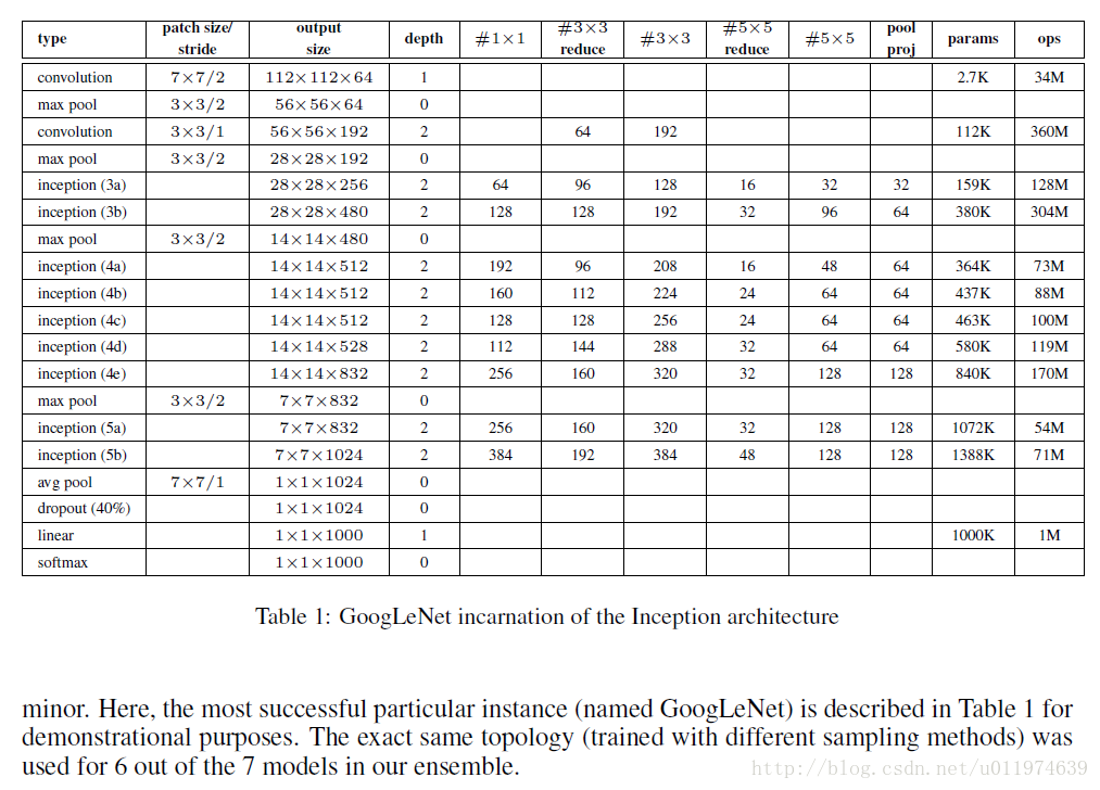
Googe Inception Net首次出现在ILSVRC2014的比赛中(和VGGNet同年)，以较大的优势获得冠军。那一届的GoogleNet通常被称为Inception V1，Inception V1的特点是控制了计算量的参数量的同时，获得了非常好的性能-top5错误率6.67%, 这主要归功于GoogleNet中引入一个新的网络结构Inception模块，所以GoogleNet又被称为Inception V1(后面还有改进版V2、V3、V4)架构中有22层深，V1比VGGNet和AlexNet都深，但是它只有500万的参数量，计算量也只有15亿次浮点运算，在参数量和计算量下降的同时保证了准确率，可以说是非常优秀并且实用的模型。

GoogleNet大家族

Google Inception Net是一个大家族,包括:

• 2014年9月的《Going deeper with convolutions》提出的Inception V1.
• 2015年2月的《Batch Normalization: Accelerating Deep Network Training by Reducing Internal Covariate Shift》提出的Inception V2
• 2015年12月的《Rethinking the Inception Architecture for Computer Vision》提出的Inception V3
• 2016年2月的《Inception-v4, Inception-ResNet and the Impact of Residual Connections on Learning》提出的Inception V4

GoogleNet的发展

Inception V1：

Inception V1中精心设计的Inception Module提高了参数的利用率；nception V1去除了模型最后的全连接层，用全局平均池化层(将图片尺寸变为1x1)，在先前的网络中，全连接层占据了网络的大部分参数，很容易产生过拟合现象；(详细见下面论文分析)

Inception V2：

Inception V2学习了VGGNet，用两个3*3的卷积代替5*5的大卷积核(降低参数量的同时减轻了过拟合)，同时还提出了注明的Batch Normalization(简称BN)方法。BN是一个非常有效的正则化方法，可以让大型卷积网络的训练速度加快很多倍，同时收敛后的分类准确率可以的到大幅度提高。

BN在用于神经网络某层时，会对每一个mini-batch数据的内部进行标准化处理，使输出规范化到(0,1)的正态分布，减少了Internal Covariate Shift(内部神经元分布的改变)。BN论文指出，传统的深度神经网络在训练时，每一层的输入的分布都在变化，导致训练变得困难，我们只能使用一个很小的学习速率解决这个问题。而对每一层使用BN之后，我们可以有效的解决这个问题，学习速率可以增大很多倍，达到之间的准确率需要的迭代次数有需要1/14，训练时间大大缩短，并且在达到之间准确率后，可以继续训练。以为BN某种意义上还起到了正则化的作用，所有可以减少或取消Dropout，简化网络结构。

当然，在使用BN时，需要一些调整：

• 增大学习率并加快学习衰减速度以适应BN规范化后的数据
• 去除Dropout并减轻L2正则(BN已起到正则化的作用)
• 去除LRN
• 更彻底地对训练样本进行shuffle
• 减少数据增强过程中对数据的光学畸变(BN训练更快，每个样本被训练的次数更少，因此真实的样本对训练更有帮助)

Inception V3：

Inception V3主要在两个方面改造:

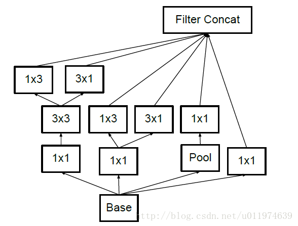
• 引入了Factorization into small convolutions的思想，将一个较大的二维卷积拆成两个较小的一位卷积，比如将7*7卷积拆成1*7卷积和7*1卷积（下图是3*3拆分为1*3和3*1的示意图）。 一方面节约了大量参数，加速运算并减去过拟合，同时增加了一层非线性扩展模型表达能力。论文中指出，这样非对称的卷积结构拆分，结果比对称地拆分为几个相同的小卷积核效果更明显，可以处理更多、更丰富的空间特征、增加特征多样性。

3*3卷积核拆分为1*3卷积和3*1卷积示意图：

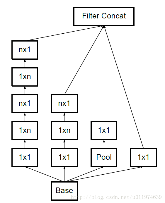
• 另一方面，Inception V3优化了Inception Module的结构，现在Inception Module有35*35、17*17和8*8三种不同的结构，如下图。这些Inception Module只在网络的后部出现，前部还是普通的卷积层。并且还在Inception Module的分支中还使用了分支。

Inception V3中三种结构的Inception Module：

• 

• 

• 

Inception V4：

Inception V4相比V3主要是结合了微软的ResNet，有兴趣的可以查看《Inception-v4, Inception-ResNet and the Impact of Residual Connections on Learning》论文。

---

GoogleNet论文分析

这里分析的是2014年9月的《Going deeper with convolutions》提出的Inception V1.

引言

原文	description
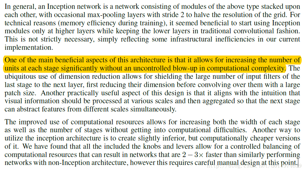
The main hallmark of this architecture is the improved utilization of the computing resources inside the network. To optimize quality, the architectural decisions were based on the Hebbian principle and the intuition of multi-scale processing	论文引入了新的网络结构Inception Modules，提高了网络内部计算资源的利用率 网络决策是基于Hebbian原理和multi-scale处理意图的

详解

将Hebbian原理应用在神经网络上，如果数据集的概率分布可以被一个很大很稀疏的神经网络表达，那么构筑这个网络的最佳方法是逐层构筑网络：将上一层高度相关的节点聚类，并将聚类出来的每一个小簇连接到一起。

1. 什么是Hebbian原理？
   神经反射活动的持续与重复会导致神经元连续稳定性持久提升，当两个神经元细胞A和B距离很近，并且A参与了对B重复、持续的兴奋，那么某些代谢会导致A将作为使B兴奋的细胞。总结一下:“一起发射的神经元会连在一起”,学习过程中的刺激会使神经元间突触强度增加。

2. 这里我们先讨论一下为什么需要稀疏的神经网络是什么概念?
   人脑神经元的连接是稀疏的，研究者认为大型神经网络的合理的连接方式应该也是稀疏的，稀疏结构是非常适合神经网络的一种结构，尤其是对非常大型、非常深的神经网络，可以减轻过拟合并降低计算量，例如CNN就是稀疏连接。

3. 为什么CNN就是稀疏连接？
   在符合Hebbian原理的基础上，我们应该把相关性高的一簇神经元节点连接在一起。在普通的数据集中，这可能需要对神经元节点做聚类，但是在图片数据中，天然的就是临近区域的数据相关性高，因此相邻的像素点被卷积操作连接在一起（符合Hebbian原理），而卷积操作就是在做稀疏连接。

4. 怎样构建满足Hebbian原理的网络？
   在CNN模型中，我们可能有多个卷积核，在同一空间位置但在不同通道的卷积核的输出结果相关性极高。我们可以使用1*1的卷积很自然的把这些相关性很高的、在同一空间位置但是不同通道的特征连接在一起。

---

1.介绍

原文

description

The biggest gains in object-detection have not come from the utilization of deep networks alone or bigger models, but from the synergy of deep architectures and classical computer vision especially their power and memory use the word “deep” is used in two different meanings: first of all, in the sense that we introduce a new level of organization in the form of the “Inception module” and also in the more direct sense of increased network depth

物体检测的最大收益并不是来自使用深层网络或更大的模型，而是来自深层架构和经典计算机视觉的协同作用 我们搭建的模型时，模型计算所需要的功耗和内存问题值得我们关注 在NIN论文中提到的deeper在本论文中有两个含义: 1.引入模块”Inception module” 2.网络的深度更深了

---

2.相关工作

原文	description
We use this approach heavily in our architecture. However, in our setting, 1 * 1 convolutions have dual purpose: most critically, they are used mainly as dimension reduction modules to remove computational bottlenecks, that would otherwise limit the size of our networks. This allows for not just increasing the depth, but also the width of our networks without significant performance penalty	我们在网络中大量使用1*1卷积核，其目的是: 使用1*1卷积核主要用来减少维度从而消除计算瓶颈，否则会限制网络的大小。使用1*1卷积核，不仅可以增加网络深度，而且还可以增加网络宽度且不会有太大的网络性能损失(功耗和内存使用不会增长过多)

---

3.动机和高层次考虑

原文

description

improving the performance of deep neural networks is by increasing their size: 1. increasing the depth 2. its width However this simple solution comes with two major drawbacks. 1.which makes the enlarged network more prone to overfitting, 2.Another drawback of uniformly increased network size is the dramatically increased use of computational resources The fundamental way of solving both issues would be by ultimately moving from fully connected to sparsely connected architectures, even inside the convolutions. Their main result states that if the probability distribution of the data-set is representable by a large, very sparse deep neural network, then the optimal network topology can be constructed layer by layer by analyzing the correlation statistics of the activations of the last layer and clustering neurons with highly correlated outputs todays computing infrastructures are very inefficient when it comes to numerical calculation on non-uniform sparse data structures

一般来说，提升网络性能最直接的方式就是增加网络的大小: 1.增加网络的深度 2.增加网络的宽度 这样简单的解决办法有两个主要的缺点: 1.网络参数的增多，网络容易陷入过拟合中，这需要大量的训练数据，而在解决高粒度分类的问题上，高质量的训练数据成本太高; 2.简单的增加网络的大小，会让网络计算量增大，而增大计算量得不到充分的利用，从而造成计算资源的浪费 解决上面的两个缺点的思路： 将全连接的结构转换为稀疏结构(即使是内部卷积) 如果数据集的概率分布可以可以有大型的稀疏的深度神经网络表示，则优化网络的方法可以是逐层的分析层输出的相关性，对相关的输出做聚类操作. 当对非均匀稀疏数据结构计算时，计算效率非常低，这需要在底层的计算库做优化;不均匀稀疏模型需要复杂的计算工程实现和设备,大多数面向视觉的机器学习系统只是利用了卷积在空间域中稀疏特性

原文

description

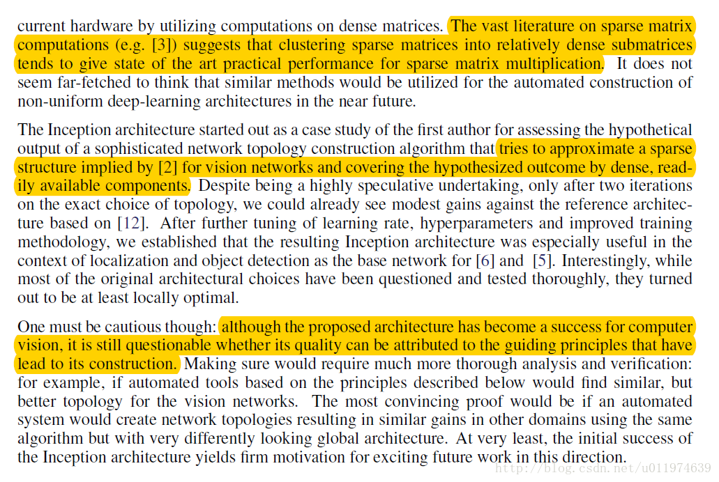
The vast literature on sparse matrix computations (e.g. [3]) suggests that clustering sparse matrices into relatively dense submatrices tends to give state of the art practical performance for sparse matrix multiplication tries to approximate a sparse structure implied by [2] for vision networks and covering the hypothesized outcome by dense, readily available components although the proposed architecture has become a success for computer vision, it is still questionable whether its quality can be attributed to the guiding principles that have lead to its construction

稀疏矩阵乘法有一个良好的实践办法是将稀疏矩阵聚类成相对密集的子矩阵 inception算法试图逼近隐含在视觉网络中的稀疏结构，并利用密集、易实现的组件来实现这样的假设(隐含的稀疏结构) 尽管提出inception这样的架构在计算机视觉上成功应用了，但是依旧存在问题：这样网络结构的性能的成功是否可以归结于网络结构的构成，这还需要探讨和验证

---

4.动机和高层次考虑

原文

description

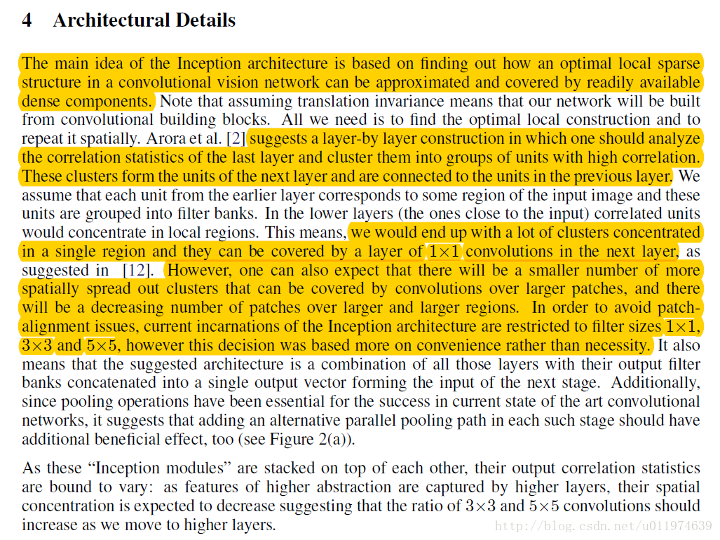
The main idea of the Inception architecture is based on finding out how an optimal local sparse structure in a convolutional vision network can be approximated and covered by readily available dense components one can also expect that there will be a smaller number of more spatially spread out clusters that can be covered by convolutions over larger patches, and there will be a decreasing number of patches over larger and larger regions. In order to avoid patchalignment issues, current incarnations of the Inception architecture are restricted to filter sizes 1*1, 3*3 and 5*5, however this decision was based more on convenience rather than necessity

inception架构的主要思想是建立在找到可以逼近的卷积视觉网络内的最优局部稀疏结构，并可以通过易实现的模块实现这种结构; 使用大的卷积核在空间上会扩散更多的区域，而对应的聚类就会变少，聚类的数目随着卷积核增大而减少，为了避免这个问题，inception架构当前只使用1*1,3*3,5*5的滤波器大小，这个决策更多的是为了方便而不是必须的。

原文

description

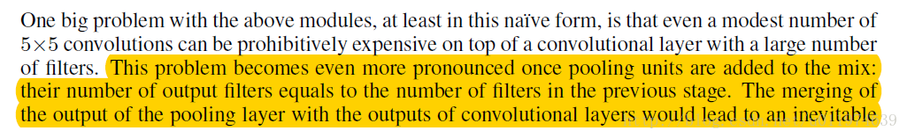
This problem becomes even more pronounced once pooling units are added to the mix: their number of output filters equals to the number of filters in the previous stage. The merging of the output of the pooling layer with the outputs of convolutional layers would lead to an inevitable increase in the number of outputs from stage to stage judiciously applying dimension reductions and projections wherever the computational requirements would increase too much otherwise 1*1 convolutions are used to compute reductions before the expensive 3*3 and 5*5 convolutions. Besides being used as reductions, they also include the use of rectified linear activation which makes them dual-purpose

将池化单元组合到一起就会面临更加明显的问题:他们输出滤波器数量等于上一阶段滤波器数量，每个阶段的跨越这就不可避免的会增加输出数量 在计算力需求急速增长的部分我们明智的应用降维和projections技术 1*1卷积做compute reductions, 而不是计算3*3或5*5的卷积;除此之外，1*1卷积还可以用来矫正线性激活

详解

我们重点关注一下Inception Module的基本结构。

Inception Module的目标即是找出易实现的，能够逼近最佳局部稀疏结构的模块，而这样的稀疏结构，是需要将层输出中相关性高的聚类到一起，这些聚类构成一下单位，与上一个单元连接。

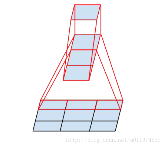
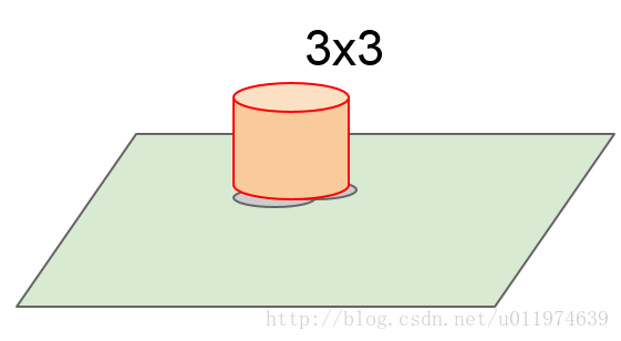
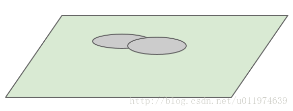
回到卷积神经网络中，假设前面层的每个单元对于于输出图像的某些区域，而卷积操作就是很好的聚类，在接近输入层的低层中，相关单元集中在某些局部区域:如下图灰色部分

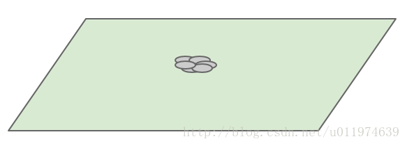
使用1*1的卷积核

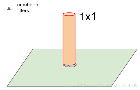
使用更大的卷积核(3*3,5*5)，使用更大的卷积核在空间上的输出会减少(维度)

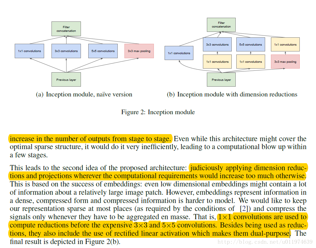
为了避免不同patch带来的校准问题，现在的滤波器大小限制在1*1，3*3和5*5，主要是为了方便。将该区域的不同卷积输出连接到一起，这样的Inception模块如下：

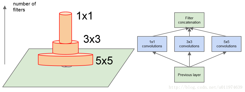
另外，添加一个额外的并行pooling路径用于提高效率

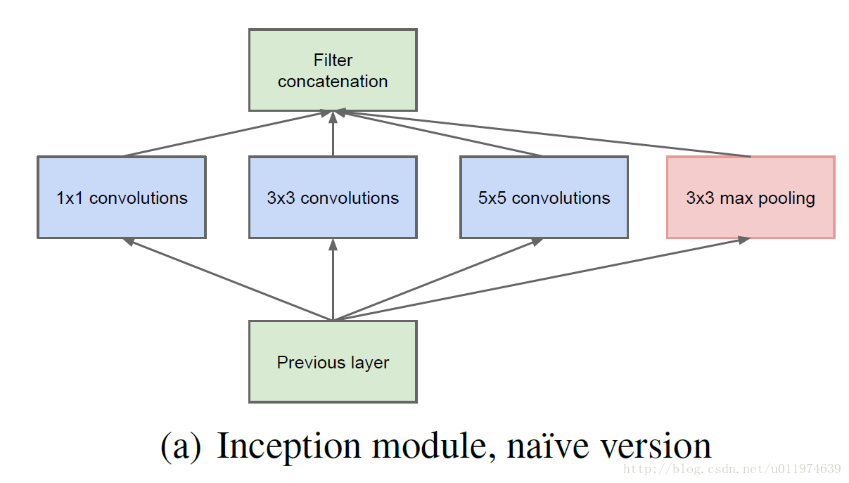
这就是Inception Module的初态了。

采用上面的结构有一个问题：
卷积层顶端由于滤波器太多，并且当pooling单元加入之后这个问题更加明显： 输出滤波器的数量等于上一步滤波器的数量。pooling层的输出和卷积层的输出融合会导致输出数量逐步增长。即使这个架构可能包含了最优的稀疏结构， 还是会非常没有效率，导致计算没经过几步就崩溃。

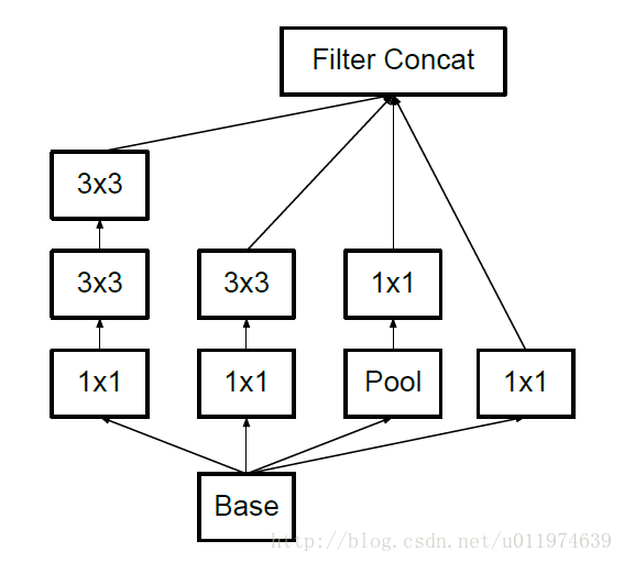
因此有了改进版的Inception Module架构：增加很多1*1的卷积操作用于降维同时也能提高网络表达能力。即在3*3和5*5的卷积前用一个1*1的卷积降维，这不仅能够减少计算，还可以修正线性激活。如下图所示。

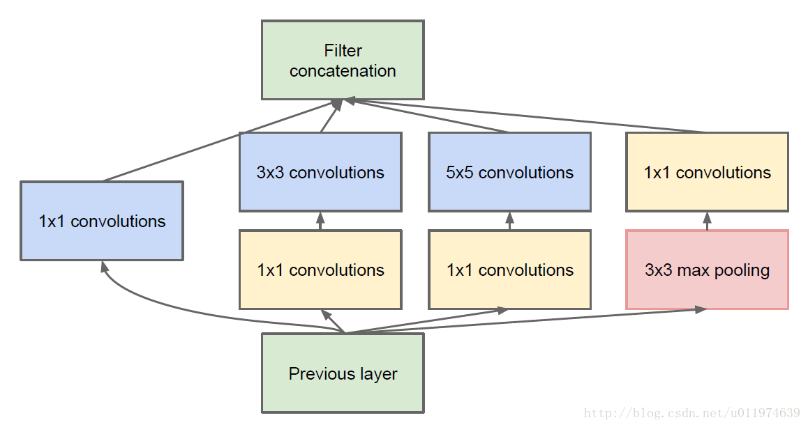
上图有4个分支: 第一个分支对输入进行1*1的卷积，1*1的卷积是一个非常优秀的结构，它可以跨通道组织信息，提高网络的表达能力，同时可以对输出通道升维或者降维；可以看到Inception Module的4个分支都用到了1*1卷积，进行低成本(计算量比3*3小很多)的跨通道的特征变换。

Inception Module的4个分支在最后通过一个聚合操作合并(在输出通道数这个维度上聚合)，构建出了很高效的符合Hebbian原理的稀疏结构。Inception Module中包含了三种不同尺寸的卷积和1个最大池化，增加了网络对不同尺度的适应性，这一部分与Multi-Scale的思想类似。总的来说Inception Module可以让网络的深度和宽度高效率地扩充，提示准确率且不致于过拟合。

在Inception Module中，通常1*1卷积的比例(输出通道数占比)最高，3*3卷积和5*5卷积稍低。整个模型中，会有多个堆叠的Inception Module，我们希望靠后的Inception Module可以捕捉更高阶的抽象特征，因此靠后的Inception Module的卷积的空间集中度应该逐渐降低，这样可以捕获更大面积的特征。因此，越靠后的Inception Module中，3*3和5*5这两个大面积的卷积核的占比(输出通道数)应该更多。

---

5.GoogLeNet

原文

description

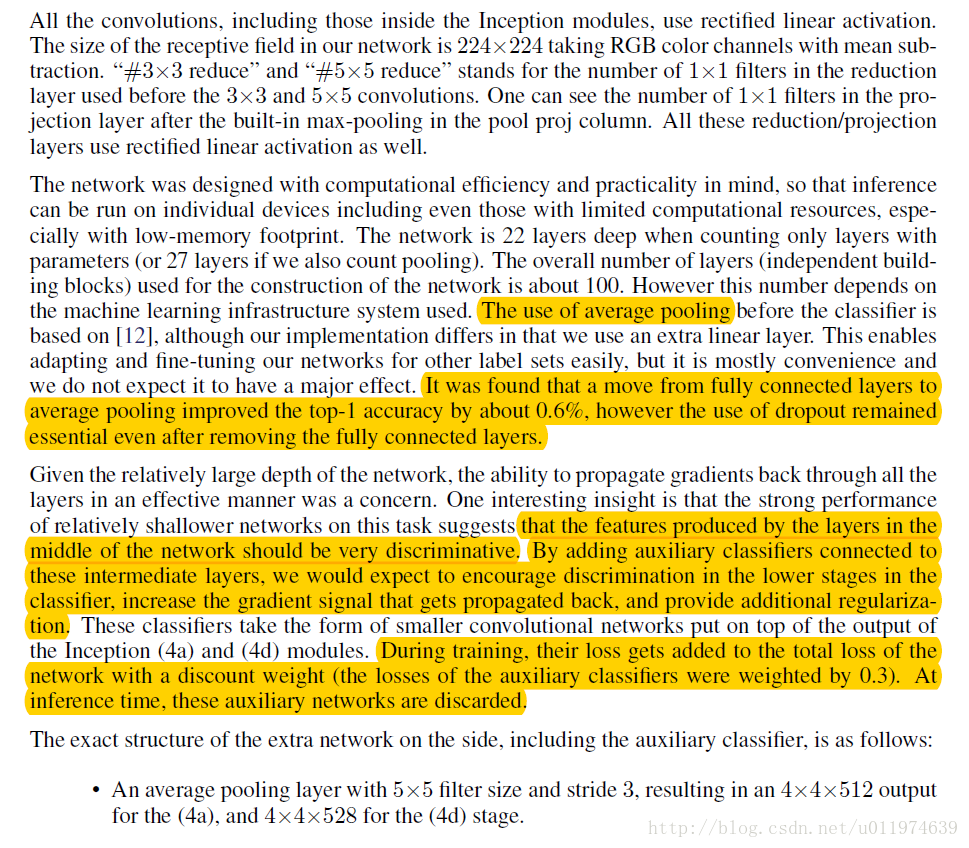
It was found that a move from fully connected layers to average pooling improved the top-1 accuracy by about 0.6%, however the use of dropout remained essential even after removing the fully connected layers. that the features produced by the layers in the middle of the network should be very discriminative By adding auxiliary classifiers connected to these intermediate layers, we would expect to encourage discrimination in the lower stages in the classifier, increase the gradient signal that gets propagated back, and provide additional regularization During training, their loss gets added to the total loss of the network with a discount weight (the losses of the auxiliary classifiers were weighted by 0.3). At inference time, these auxiliary networks are discarded.

使用平均池化代替FC层可以提高top-1精度0.6%,需要注意的是即使是移除掉了FC层，仍需要使用dropout技术 有一个很好的观点：网络的中间层应该是很有判别力的(考虑到网络深度有22层，且有一些浅层的模型表现的很好) 我们期望分类器可以在较低阶段就可以区分，故在网络的中间层添加了辅助分类器，这不仅可以在BP中增加传播的梯度信号，而且可以提供额外的正则化 在训练过程中，辅助分类器的loss也计算到总的loss中，loss以不同比例的权重计算(占比为0.3)，在inference阶段，辅助分类器不使用

详解

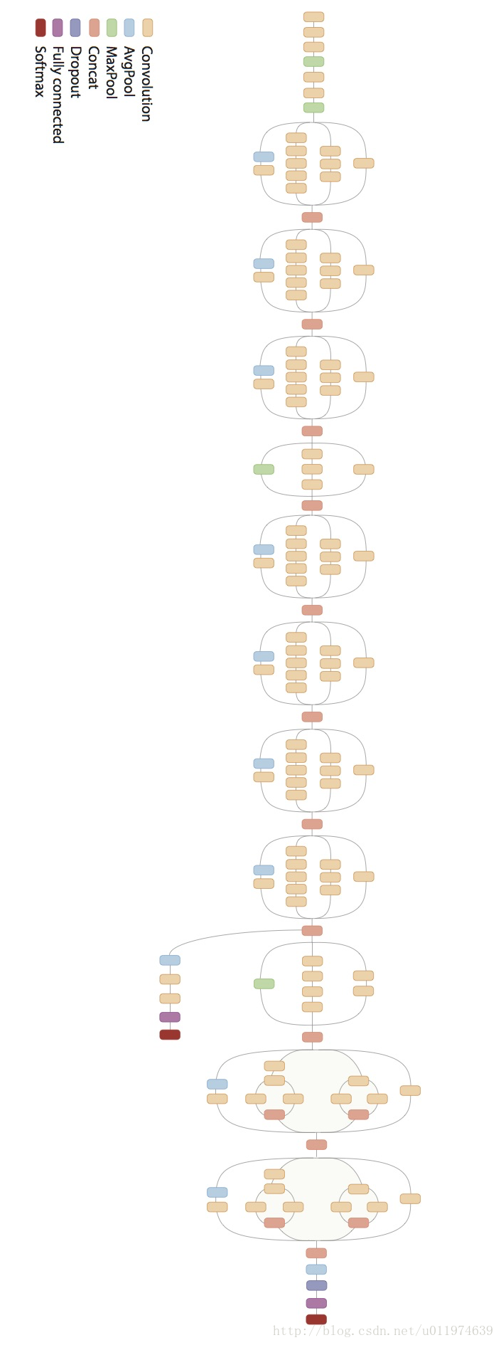
GoogleNet整个网络架构如下图所示:

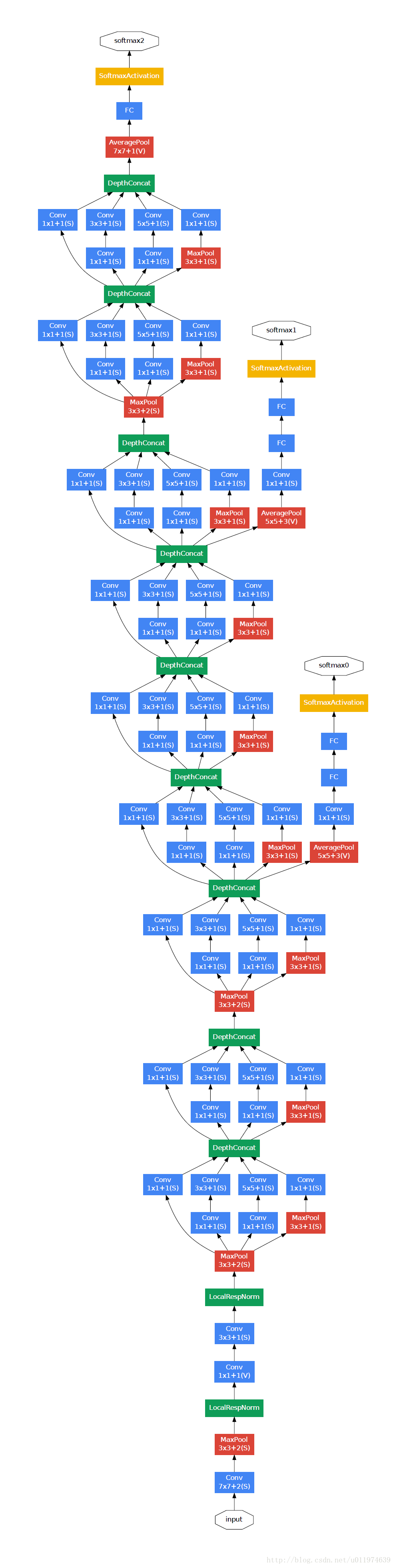
对于辅助分类器：

Inception Net 有22层深，除了最后一层的输出，其中间节点的分类效果也很好，因此在Inception Net中， 还使用了辅助分类节点(auxiliary classifiers)，即将中间某一层的输出用作分类，并按一个较小的权重(0.3)加到最终分类结果中，这样相当于做了模型融合，同时给网络增加了BP的梯度信号，也提供了额外的正则化。

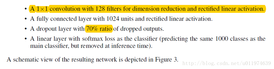
辅助分类器结构：

1. 均值pooling层滤波器大小为5*5，步长为3，(4a)的输出为4*4*512，(4d)的输出为4*4*528；
2. 有128个1*1的卷积用于降维和修正线性激活；
3. 全连接层有1024个单元和修正线性激活；
4. dropout层比率为70%；
5. 线性层将softmax损失作为分类器（和主分类器一样预测1000个类，但在inference时移除）。

---

6.训练方法

原文	description
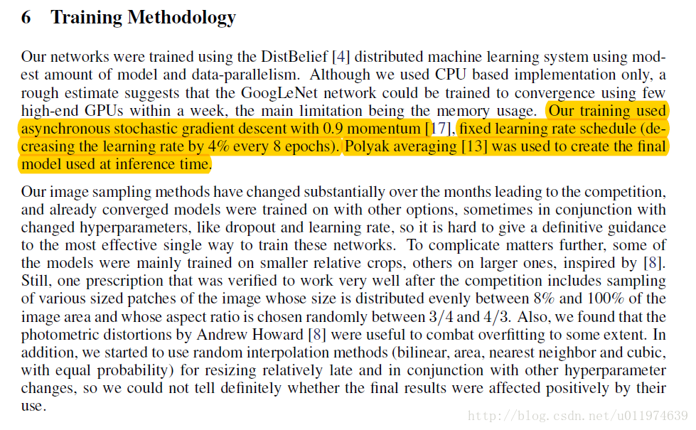
Our training used asynchronous stochastic gradient descent with 0.9 momentum [17], fixed learning rate schedule (decreasing he learning rate by 4% every 8 epochs). Polyak averaging [13] was used to create the final model used at inference time	训练使用带0.9动量的异步随机梯度下降法，学习率是固定的变化的(每8个epochs下降4%)，在inference 时候我们使用Polyak averaging 来创建最终模型

---

7.ILSVRC 2014 Classification Challenge Setup and Results

原文

description

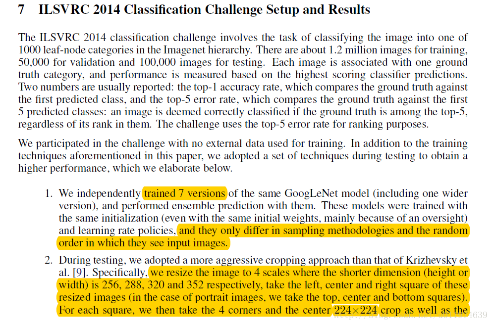
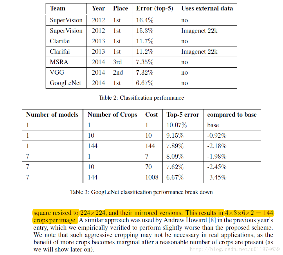
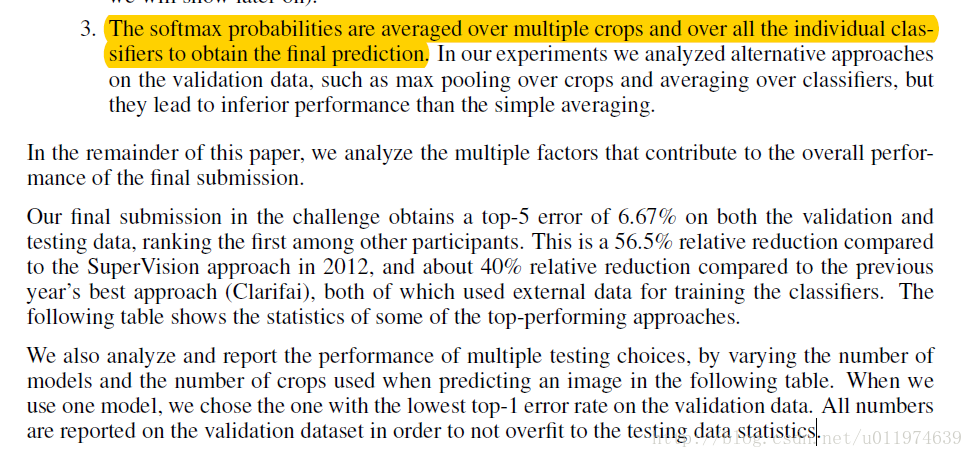
We independently trained 7 versions of the same GoogLeNet model and they only differ in sampling methodologies and the random order in which they see input images. 2. we resize the image to 4 scales where the shorter dimension (height or width) is 256, 288, 320 and 352 respectively, take the left, center and right square of these resized images (in the case of portrait images, we take the top, center and bottom squares). For each square, we then take the 4 corners and the center 224*224 crop as well as the square resized to 224*224, and their mirrored versions. This results in 4*3*6*2 = 144 crops per image The softmax probabilities are averaged over multiple crops and over all the individual classifiers to obtain the final prediction.

分别训练了7个模型,每个模型的初试操作相同(相同的初试权值),不同的是每个模型的采样方法和随机输入图片 在测试时，将图片的短边resize到4个代表性的大小(256,288,320,352),在分别在取出resized那边的上中下(左中右)三个正方形区域，每个正方形区域取出五个区域(左上、右上、左下、右下、中央)，再将正方形区域resize到224大小，一共是6个图片，再水平翻转一次，一共是4*3*6*2 = 144张测试图片 最终输出在softmax层做平均，获得最终的预测

---

8.ILSVRC 2014 Detection Challenge Setup and Results

（略）

9.总结

（略）….

---

---

GoogleNet在TensorFlow的实现

由于Google Inception Net相对比较复杂，我们模仿着在TensorFlow的GitHub代码库上开源的Inception-V3模型的源码，V3模型中使用的Inception模型相比V1和V2有着更加复杂多样的网络结构；

V3模型共有46层，有三个Inception模型组(三层、五层、三层)，共有96的卷积层，可以想象V3的代码会很长，这里使用tf.contrib.slim工具辅助设计网络， 简化代码。

V3的网络架构图如下：

网络总览:

类型	kernel尺寸/步长(或注释)	输出尺寸
conv0	3 * 3 / 2	149 * 149 * 32
conv1	3 * 3 / 1	147 * 147 * 32
conv2	3 * 3 / 1	147 * 147 * 64
pool1	3 * 3 / 2	73 * 73 * 64
conv3	3 * 3 / 1	73 * 73 * 80
conv4	3 * 3 / 1	71 * 71 * 192
pool2	3 * 3 / 2	35 * 35 * 192
Inception模块	mixed_b mixed_c mixed_d	35 * 35 * 256 35 * 35 * 288 35 * 35 * 288
Inception模块	mixed_a mixed_b mixed_c mixed_d mixed_e	17 * 17 * 768 17 * 17 * 768 17 * 17 * 768 17 * 17 * 768 17 * 17 * 768
Inception模块	mixed_a mixed_b mixed_c	8 * 8 * 1280 8 * 8 * 2048 8 * 8 * 2048
池化	8 * 8	1 * 1 * 2048
logits	logits	1 * 1 * 1000
Softmax	分类输出	1 * 1 * 1000
辅助分类器
avg_pool	5 * 5 / 3	5 * 5 * 768
conv0	1 * 1 / 1	5 * 5 * 128
conv1	5 * 5 / 1	1 * 1 * 768
logits	logits	1 * 1 * 1000

---

代码实现如下（所以设计和尺寸参见注释）:

# coding:UTF-8
import tensorflow as tf
from datetime import datetime
import math
import time

slim = tf.contrib.slim
trunc_normal = lambda stddev: tf.truncated_normal_initializer(0.0, stddev)

# 用来生成网络中经常用到的函数的默认参数
# 默认参数：卷积的激活函数、权重初始化方式、标准化器等
def inception_v3_arg_scope(weight_decay=0.00004,    # L2正则的weight_decay
                           stddev=0.1,  # 标准差0.1
                           batch_norm_var_collection='moving_vars'):

  batch_norm_params = {  # 定义batch normalization参数字典
      'decay': 0.9997,  #衰减系数
      'epsilon': 0.001,
      'updates_collections': tf.GraphKeys.UPDATE_OPS,
      'variables_collections': {
          'beta': None,
          'gamma': None,
          'moving_mean': [batch_norm_var_collection],
          'moving_variance': [batch_norm_var_collection],
      }
  }

  # silm.arg_scope可以给函数自动赋予某些默认值
  # 会对[slim.conv2d, slim.fully_connected]这两个函数的参数自动赋值,
  # 使用slim.arg_scope后就不需要每次都重复设置参数了，只需要在有修改时设置
  with slim.arg_scope([slim.conv2d, slim.fully_connected],
                      weights_regularizer=slim.l2_regularizer(weight_decay)): # 对[slim.conv2d, slim.fully_connected]自动赋值

      # 嵌套一个slim.arg_scope对卷积层生成函数slim.conv2d的几个参数赋予默认值
    with slim.arg_scope(
        [slim.conv2d],
        weights_initializer=trunc_normal(stddev), # 权重初始化器
        activation_fn=tf.nn.relu, # 激活函数
        normalizer_fn=slim.batch_norm, # 标准化器
        normalizer_params=batch_norm_params) as sc: # 标准化器的参数设置为前面定义的batch_norm_params
      return sc # 最后返回定义好的scope




# 生成V3网络的卷积部分
def inception_v3_base(inputs, scope=None):
  '''
  Args:
  inputs：输入的tensor
  scope：包含了函数默认参数的环境
  '''
  end_points = {} # 定义一个字典表保存某些关键节点供之后使用

  with tf.variable_scope(scope, 'InceptionV3', [inputs]):
    with slim.arg_scope([slim.conv2d, slim.max_pool2d, slim.avg_pool2d], # 对三个参数设置默认值
                        stride=1, padding='VALID'):

      #  因为使用了slim以及slim.arg_scope，我们一行代码就可以定义好一个卷积层
      #  相比AlexNet使用好几行代码定义一个卷积层，或是VGGNet中专门写一个函数定义卷积层，都更加方便
      #
      # 正式定义Inception V3的网络结构。首先是前面的非Inception Module的卷积层
      # slim.conv2d函数第一个参数为输入的tensor，第二个是输出的通道数，卷积核尺寸，步长stride，padding模式

      #一共有5个卷积层，2个池化层，实现了对图片数据的尺寸压缩，并对图片特征进行了抽象
      # 299 x 299 x 3
      net = slim.conv2d(inputs, 32, [3, 3],
                        stride=2, scope='Conv2d_1a_3x3')    # 149 x 149 x 32

      net = slim.conv2d(net, 32, [3, 3],
                        scope='Conv2d_2a_3x3')      # 147 x 147 x 32

      net = slim.conv2d(net, 64, [3, 3], padding='SAME',
                        scope='Conv2d_2b_3x3')  # 147 x 147 x 64

      net = slim.max_pool2d(net, [3, 3], stride=2,
                            scope='MaxPool_3a_3x3')   # 73 x 73 x 64

      net = slim.conv2d(net, 80, [1, 1],
                        scope='Conv2d_3b_1x1')  # 73 x 73 x 80

      net = slim.conv2d(net, 192, [3, 3],
                        scope='Conv2d_4a_3x3')  # 71 x 71 x 192

      net = slim.max_pool2d(net, [3, 3], stride=2,
                            scope='MaxPool_5a_3x3') # 35 x 35 x 192


    '''
    三个连续的Inception模块组，三个Inception模块组中各自分别有多个Inception Module，这部分是Inception Module V3
    的精华所在。每个Inception模块组内部的几个Inception Mdoule结构非常相似，但是存在一些细节的不同
    '''
    # Inception blocks
    with slim.arg_scope([slim.conv2d, slim.max_pool2d, slim.avg_pool2d], # 设置所有模块组的默认参数
                        stride=1, padding='SAME'): # 将所有卷积层、最大池化、平均池化层步长都设置为1
      # 第一个模块组包含了三个结构类似的Inception Module
      '''    
--------------------------------------------------------    
      第一个Inception组   一共三个Inception模块
      '''
      with tf.variable_scope('Mixed_5b'): # 第一个Inception Module名称。Inception Module有四个分支
        # 第一个分支64通道的1*1卷积
        with tf.variable_scope('Branch_0'):
          branch_0 = slim.conv2d(net, 64, [1, 1], scope='Conv2d_0a_1x1') # 35x35x64

        # 第二个分支48通道1*1卷积，链接一个64通道的5*5卷积
        with tf.variable_scope('Branch_1'):
          branch_1 = slim.conv2d(net, 48, [1, 1], scope='Conv2d_0a_1x1') # 35x35x48
          branch_1 = slim.conv2d(branch_1, 64, [5, 5], scope='Conv2d_0b_5x5') #35x35x64

        # 第三个分支64通道1*1卷积,96的3*3,再接一个3*3
        with tf.variable_scope('Branch_2'):
          branch_2 = slim.conv2d(net, 64, [1, 1], scope='Conv2d_0a_1x1')
          branch_2 = slim.conv2d(branch_2, 96, [3, 3], scope='Conv2d_0b_3x3')
          branch_2 = slim.conv2d(branch_2, 96, [3, 3], scope='Conv2d_0c_3x3')#35x35x96

        # 第四个分支64通道3*3平均池化,32的1*1
        with tf.variable_scope('Branch_3'):
          branch_3 = slim.avg_pool2d(net, [3, 3], scope='AvgPool_0a_3x3')
          branch_3 = slim.conv2d(branch_3, 32, [1, 1], scope='Conv2d_0b_1x1') #35*35*32
        net = tf.concat([branch_0, branch_1, branch_2, branch_3], 3) # 将四个分支的输出合并在一起（第三个维度合并，即输出通道上合并）
      # 64+64+96+32 = 256
      # mixed_1: 35 x 35 x 256.
      '''
      因为这里所有层步长均为1，并且padding模式为SAME，所以图片尺寸不会缩小，但是通道数增加了。四个分支通道数之和
      64+64+96+32=256，最终输出的tensor的图片尺寸为35*35*256
      '''

      with tf.variable_scope('Mixed_5c'):
        with tf.variable_scope('Branch_0'):
          branch_0 = slim.conv2d(net, 64, [1, 1], scope='Conv2d_0a_1x1')
        with tf.variable_scope('Branch_1'):
          branch_1 = slim.conv2d(net, 48, [1, 1], scope='Conv2d_0b_1x1')
          branch_1 = slim.conv2d(branch_1, 64, [5, 5], scope='Conv_1_0c_5x5')
        with tf.variable_scope('Branch_2'):
          branch_2 = slim.conv2d(net, 64, [1, 1], scope='Conv2d_0a_1x1')
          branch_2 = slim.conv2d(branch_2, 96, [3, 3], scope='Conv2d_0b_3x3')
          branch_2 = slim.conv2d(branch_2, 96, [3, 3], scope='Conv2d_0c_3x3')
        with tf.variable_scope('Branch_3'):
          branch_3 = slim.avg_pool2d(net, [3, 3], scope='AvgPool_0a_3x3')
          branch_3 = slim.conv2d(branch_3, 64, [1, 1], scope='Conv2d_0b_1x1')
        net = tf.concat([branch_0, branch_1, branch_2, branch_3], 3)
      # 64+64+96+64 = 288
      # mixed_2: 35 x 35 x 288.

      with tf.variable_scope('Mixed_5d'):
        with tf.variable_scope('Branch_0'):
          branch_0 = slim.conv2d(net, 64, [1, 1], scope='Conv2d_0a_1x1')
        with tf.variable_scope('Branch_1'):
          branch_1 = slim.conv2d(net, 48, [1, 1], scope='Conv2d_0a_1x1')
          branch_1 = slim.conv2d(branch_1, 64, [5, 5], scope='Conv2d_0b_5x5')
        with tf.variable_scope('Branch_2'):
          branch_2 = slim.conv2d(net, 64, [1, 1], scope='Conv2d_0a_1x1')
          branch_2 = slim.conv2d(branch_2, 96, [3, 3], scope='Conv2d_0b_3x3')
          branch_2 = slim.conv2d(branch_2, 96, [3, 3], scope='Conv2d_0c_3x3')
        with tf.variable_scope('Branch_3'):
          branch_3 = slim.avg_pool2d(net, [3, 3], scope='AvgPool_0a_3x3')
          branch_3 = slim.conv2d(branch_3, 64, [1, 1], scope='Conv2d_0b_1x1')
        net = tf.concat([branch_0, branch_1, branch_2, branch_3], 3)

      # 64+64+96+64 = 288
      # mixed_1: 35 x 35 x 288

        '''    
        第一个Inception组结束  一共三个Inception模块 输出为:35*35*288
----------------------------------------------------------------------    
        第二个Inception组   共5个Inception模块
        '''

      with tf.variable_scope('Mixed_6a'):
        with tf.variable_scope('Branch_0'):
          branch_0 = slim.conv2d(net, 384, [3, 3], stride=2,
                                 padding='VALID', scope='Conv2d_1a_1x1') #17*17*384
        with tf.variable_scope('Branch_1'):
          branch_1 = slim.conv2d(net, 64, [1, 1], scope='Conv2d_0a_1x1') #35*35*64
          branch_1 = slim.conv2d(branch_1, 96, [3, 3], scope='Conv2d_0b_3x3')#35*35*96
          branch_1 = slim.conv2d(branch_1, 96, [3, 3], stride=2,
                                 padding='VALID', scope='Conv2d_1a_1x1') #17*17*96
        with tf.variable_scope('Branch_2'):
          branch_2 = slim.max_pool2d(net, [3, 3], stride=2, padding='VALID',
                                     scope='MaxPool_1a_3x3') #17*17*288
        net = tf.concat([branch_0, branch_1, branch_2], 3) # 输出尺寸定格在17 x 17 x 768
      # 384+96+288 = 768
      # mixed_3: 17 x 17 x 768.

      with tf.variable_scope('Mixed_6b'):
        with tf.variable_scope('Branch_0'):
          branch_0 = slim.conv2d(net, 192, [1, 1], scope='Conv2d_0a_1x1')
        with tf.variable_scope('Branch_1'):
          branch_1 = slim.conv2d(net, 128, [1, 1], scope='Conv2d_0a_1x1')
          branch_1 = slim.conv2d(branch_1, 128, [1, 7], scope='Conv2d_0b_1x7') # 串联1*7卷积和7*1卷积合成7*7卷积，减少了参数，减轻了过拟合
          branch_1 = slim.conv2d(branch_1, 192, [7, 1], scope='Conv2d_0c_7x1')
        with tf.variable_scope('Branch_2'):
          branch_2 = slim.conv2d(net, 128, [1, 1], scope='Conv2d_0a_1x1') # 反复将7*7卷积拆分
          branch_2 = slim.conv2d(branch_2, 128, [7, 1], scope='Conv2d_0b_7x1')
          branch_2 = slim.conv2d(branch_2, 128, [1, 7], scope='Conv2d_0c_1x7')
          branch_2 = slim.conv2d(branch_2, 128, [7, 1], scope='Conv2d_0d_7x1')
          branch_2 = slim.conv2d(branch_2, 192, [1, 7], scope='Conv2d_0e_1x7')
        with tf.variable_scope('Branch_3'):
          branch_3 = slim.avg_pool2d(net, [3, 3], scope='AvgPool_0a_3x3')
          branch_3 = slim.conv2d(branch_3, 192, [1, 1], scope='Conv2d_0b_1x1')
        net = tf.concat([branch_0, branch_1, branch_2, branch_3], 3)
      # 192+192+192+192 = 768
      # mixed4: 17 x 17 x 768.


      with tf.variable_scope('Mixed_6c'):
        with tf.variable_scope('Branch_0'):
          '''
          我们的网络每经过一个inception module，即使输出尺寸不变，但是特征都相当于被重新精炼了一遍，
          其中丰富的卷积和非线性化对提升网络性能帮助很大。
          '''
          branch_0 = slim.conv2d(net, 192, [1, 1], scope='Conv2d_0a_1x1')
        with tf.variable_scope('Branch_1'):
          branch_1 = slim.conv2d(net, 160, [1, 1], scope='Conv2d_0a_1x1')
          branch_1 = slim.conv2d(branch_1, 160, [1, 7], scope='Conv2d_0b_1x7')
          branch_1 = slim.conv2d(branch_1, 192, [7, 1], scope='Conv2d_0c_7x1')
        with tf.variable_scope('Branch_2'):
          branch_2 = slim.conv2d(net, 160, [1, 1], scope='Conv2d_0a_1x1')
          branch_2 = slim.conv2d(branch_2, 160, [7, 1], scope='Conv2d_0b_7x1')
          branch_2 = slim.conv2d(branch_2, 160, [1, 7], scope='Conv2d_0c_1x7')
          branch_2 = slim.conv2d(branch_2, 160, [7, 1], scope='Conv2d_0d_7x1')
          branch_2 = slim.conv2d(branch_2, 192, [1, 7], scope='Conv2d_0e_1x7')
        with tf.variable_scope('Branch_3'):
          branch_3 = slim.avg_pool2d(net, [3, 3], scope='AvgPool_0a_3x3')
          branch_3 = slim.conv2d(branch_3, 192, [1, 1], scope='Conv2d_0b_1x1')
        net = tf.concat([branch_0, branch_1, branch_2, branch_3], 3)
      # 192+192+192+192 = 768
      # mixed_5: 17 x 17 x 768.


      with tf.variable_scope('Mixed_6d'):
        with tf.variable_scope('Branch_0'):
          branch_0 = slim.conv2d(net, 192, [1, 1], scope='Conv2d_0a_1x1')
        with tf.variable_scope('Branch_1'):
          branch_1 = slim.conv2d(net, 160, [1, 1], scope='Conv2d_0a_1x1')
          branch_1 = slim.conv2d(branch_1, 160, [1, 7], scope='Conv2d_0b_1x7')
          branch_1 = slim.conv2d(branch_1, 192, [7, 1], scope='Conv2d_0c_7x1')
        with tf.variable_scope('Branch_2'):
          branch_2 = slim.conv2d(net, 160, [1, 1], scope='Conv2d_0a_1x1')
          branch_2 = slim.conv2d(branch_2, 160, [7, 1], scope='Conv2d_0b_7x1')
          branch_2 = slim.conv2d(branch_2, 160, [1, 7], scope='Conv2d_0c_1x7')
          branch_2 = slim.conv2d(branch_2, 160, [7, 1], scope='Conv2d_0d_7x1')
          branch_2 = slim.conv2d(branch_2, 192, [1, 7], scope='Conv2d_0e_1x7')
        with tf.variable_scope('Branch_3'):
          branch_3 = slim.avg_pool2d(net, [3, 3], scope='AvgPool_0a_3x3')
          branch_3 = slim.conv2d(branch_3, 192, [1, 1], scope='Conv2d_0b_1x1')
        net = tf.concat([branch_0, branch_1, branch_2, branch_3], 3)
      # 92+192+192+192 = 768
      # mixed_6: 17 x 17 x 768.

      with tf.variable_scope('Mixed_6e'):
        with tf.variable_scope('Branch_0'):
          branch_0 = slim.conv2d(net, 192, [1, 1], scope='Conv2d_0a_1x1')
        with tf.variable_scope('Branch_1'):
          branch_1 = slim.conv2d(net, 192, [1, 1], scope='Conv2d_0a_1x1')
          branch_1 = slim.conv2d(branch_1, 192, [1, 7], scope='Conv2d_0b_1x7')
          branch_1 = slim.conv2d(branch_1, 192, [7, 1], scope='Conv2d_0c_7x1')
        with tf.variable_scope('Branch_2'):
          branch_2 = slim.conv2d(net, 192, [1, 1], scope='Conv2d_0a_1x1')
          branch_2 = slim.conv2d(branch_2, 192, [7, 1], scope='Conv2d_0b_7x1')
          branch_2 = slim.conv2d(branch_2, 192, [1, 7], scope='Conv2d_0c_1x7')
          branch_2 = slim.conv2d(branch_2, 192, [7, 1], scope='Conv2d_0d_7x1')
          branch_2 = slim.conv2d(branch_2, 192, [1, 7], scope='Conv2d_0e_1x7')
        with tf.variable_scope('Branch_3'):
          branch_3 = slim.avg_pool2d(net, [3, 3], scope='AvgPool_0a_3x3')
          branch_3 = slim.conv2d(branch_3, 192, [1, 1], scope='Conv2d_0b_1x1')
        net = tf.concat([branch_0, branch_1, branch_2, branch_3], 3)
      # 92+192+192+192 = 768
      # mixed_7: 17 x 17 x 768.


        '''    
        第二个Inception组结束  一共五个Inception模块 输出为:17*17*768
----------------------------------------------------------------------    
        第三个Inception组   共3个Inception模块(带分支)
        '''
      # 将Mixed_6e存储于end_points中，作为Auxiliary Classifier辅助模型的分类
      end_points['Mixed_6e'] = net

      # 第三个inception模块组包含了三个inception module

      with tf.variable_scope('Mixed_7a'):
        with tf.variable_scope('Branch_0'):
          branch_0 = slim.conv2d(net, 192, [1, 1], scope='Conv2d_0a_1x1')# 17*17*192
          branch_0 = slim.conv2d(branch_0, 320, [3, 3], stride=2,
                                 padding='VALID', scope='Conv2d_1a_3x3') # 8*8*320
        with tf.variable_scope('Branch_1'):
          branch_1 = slim.conv2d(net, 192, [1, 1], scope='Conv2d_0a_1x1') #17*17*192
          branch_1 = slim.conv2d(branch_1, 192, [1, 7], scope='Conv2d_0b_1x7')
          branch_1 = slim.conv2d(branch_1, 192, [7, 1], scope='Conv2d_0c_7x1')
          branch_1 = slim.conv2d(branch_1, 192, [3, 3], stride=2,
                                 padding='VALID', scope='Conv2d_1a_3x3') #8*8*192
        with tf.variable_scope('Branch_2'):
          branch_2 = slim.max_pool2d(net, [3, 3], stride=2, padding='VALID',
                                     scope='MaxPool_1a_3x3')  #8*8*768
        net = tf.concat([branch_0, branch_1, branch_2], 3) # 输出图片尺寸被缩小，通道数增加，tensor的总size在持续下降中
      # 320+192+768 = 1280
      # mixed_8: 8 x 8 x 1280.


      with tf.variable_scope('Mixed_7b'):
        with tf.variable_scope('Branch_0'):
          branch_0 = slim.conv2d(net, 320, [1, 1], scope='Conv2d_0a_1x1')
        with tf.variable_scope('Branch_1'):
          branch_1 = slim.conv2d(net, 384, [1, 1], scope='Conv2d_0a_1x1')
          branch_1 = tf.concat([
              slim.conv2d(branch_1, 384, [1, 3], scope='Conv2d_0b_1x3'),
              slim.conv2d(branch_1, 384, [3, 1], scope='Conv2d_0b_3x1')], 3)
        with tf.variable_scope('Branch_2'):
          branch_2 = slim.conv2d(net, 448, [1, 1], scope='Conv2d_0a_1x1')
          branch_2 = slim.conv2d(branch_2, 384, [3, 3], scope='Conv2d_0b_3x3')
          branch_2 = tf.concat([
              slim.conv2d(branch_2, 384, [1, 3], scope='Conv2d_0c_1x3'),
              slim.conv2d(branch_2, 384, [3, 1], scope='Conv2d_0d_3x1')], 3)
        with tf.variable_scope('Branch_3'):
          branch_3 = slim.avg_pool2d(net, [3, 3], scope='AvgPool_0a_3x3')
          branch_3 = slim.conv2d(branch_3, 192, [1, 1], scope='Conv2d_0b_1x1')
        net = tf.concat([branch_0, branch_1, branch_2, branch_3], 3) # 输出通道数增加到2048
      # 320+(384+384)+(384+384)+192 = 2048
      # mixed_9: 8 x 8 x 2048.



      with tf.variable_scope('Mixed_7c'):
        with tf.variable_scope('Branch_0'):
          branch_0 = slim.conv2d(net, 320, [1, 1], scope='Conv2d_0a_1x1')
        with tf.variable_scope('Branch_1'):
          branch_1 = slim.conv2d(net, 384, [1, 1], scope='Conv2d_0a_1x1')
          branch_1 = tf.concat([
              slim.conv2d(branch_1, 384, [1, 3], scope='Conv2d_0b_1x3'),
              slim.conv2d(branch_1, 384, [3, 1], scope='Conv2d_0c_3x1')], 3)
        with tf.variable_scope('Branch_2'):
          branch_2 = slim.conv2d(net, 448, [1, 1], scope='Conv2d_0a_1x1')
          branch_2 = slim.conv2d(branch_2, 384, [3, 3], scope='Conv2d_0b_3x3')
          branch_2 = tf.concat([
              slim.conv2d(branch_2, 384, [1, 3], scope='Conv2d_0c_1x3'),
              slim.conv2d(branch_2, 384, [3, 1], scope='Conv2d_0d_3x1')], 3)
        with tf.variable_scope('Branch_3'):
          branch_3 = slim.avg_pool2d(net, [3, 3], scope='AvgPool_0a_3x3')
          branch_3 = slim.conv2d(branch_3, 192, [1, 1], scope='Conv2d_0b_1x1')
        net = tf.concat([branch_0, branch_1, branch_2, branch_3], 3)
      # 320+(384+384)+(384+384)+192 = 2048
      # mixed_10: 8 x 8 x 2048.

      return net, end_points
      #Inception V3网络的核心部分，即卷积层部分就完成了
      '''
      设计inception net的重要原则是图片尺寸不断缩小，inception模块组的目的都是将空间结构简化，同时将空间信息转化为
      高阶抽象的特征信息，即将空间维度转为通道的维度。降低了计算量。Inception Module是通过组合比较简单的特征
      抽象（分支1）、比较比较复杂的特征抽象（分支2和分支3）和一个简化结构的池化层（分支4），一共四种不同程度的
      特征抽象和变换来有选择地保留不同层次的高阶特征，这样最大程度地丰富网络的表达能力。
      '''



# V3最后部分
# 全局平均池化、Softmax和Auxiliary Logits
def inception_v3(inputs,
                 num_classes=1000, # 最后需要分类的数量（比赛数据集的种类数）
                 is_training=True, # 标志是否为训练过程，只有在训练时Batch normalization和Dropout才会启用
                 dropout_keep_prob=0.8, # 节点保留比率
                 prediction_fn=slim.softmax, # 最后用来分类的函数
                 spatial_squeeze=True, # 参数标志是否对输出进行squeeze操作（去除维度数为1的维度，比如5*3*1转为5*3）
                 reuse=None, # 是否对网络和Variable进行重复使用
                 scope='InceptionV3'): # 包含函数默认参数的环境

  with tf.variable_scope(scope, 'InceptionV3', [inputs, num_classes], # 定义参数默认值
                         reuse=reuse) as scope:
    with slim.arg_scope([slim.batch_norm, slim.dropout], # 定义标志默认值
                        is_training=is_training):
      # 拿到最后一层的输出net和重要节点的字典表end_points
      net, end_points = inception_v3_base(inputs, scope=scope) # 用定义好的函数构筑整个网络的卷积部分

      # Auxiliary logits作为辅助分类的节点，对分类结果预测有很大帮助
      with slim.arg_scope([slim.conv2d, slim.max_pool2d, slim.avg_pool2d],
                          stride=1, padding='SAME'): # 将卷积、最大池化、平均池化步长设置为1
        aux_logits = end_points['Mixed_6e'] # 通过end_points取到Mixed_6e
        # end_points['Mixed_6e']  --> 17x17x768
        with tf.variable_scope('AuxLogits'):
          aux_logits = slim.avg_pool2d(
                    aux_logits, [5, 5], stride=3, padding='VALID',
                    scope='AvgPool_1a_5x5') #5x5x768

          aux_logits = slim.conv2d(aux_logits, 128, [1, 1],
                                   scope='Conv2d_1b_1x1') #5x5x128

          # Shape of feature map before the final layer.
          aux_logits = slim.conv2d(
              aux_logits, 768, [5, 5],
              weights_initializer=trunc_normal(0.01),
              padding='VALID', scope='Conv2d_2a_5x5')  #1x1x768

          aux_logits = slim.conv2d(
              aux_logits, num_classes, [1, 1], activation_fn=None,
              normalizer_fn=None, weights_initializer=trunc_normal(0.001),
              scope='Conv2d_2b_1x1')  # 1*1*1000

          if spatial_squeeze: # tf.squeeze消除tensor中前两个为1的维度。
            aux_logits = tf.squeeze(aux_logits, [1, 2], name='SpatialSqueeze')
          end_points['AuxLogits'] = aux_logits # 最后将辅助分类节点的输出aux_logits储存到字典表end_points中

      # 处理正常的分类预测逻辑
      # Final pooling and prediction
      with tf.variable_scope('Logits'):
        # net --> 8x8x2048
        net = slim.avg_pool2d(net, [8, 8], padding='VALID',
                              scope='AvgPool_1a_8x8') #1x1x2048

        net = slim.dropout(net, keep_prob=dropout_keep_prob, scope='Dropout_1b')
        end_points['PreLogits'] = net

        # 激活函数和规范化函数设为空
        logits = slim.conv2d(net, num_classes, [1, 1], activation_fn=None,
                             normalizer_fn=None, scope='Conv2d_1c_1x1') # 1x1x1000
        if spatial_squeeze: # tf.squeeze去除输出tensor中维度为1的节点
          logits = tf.squeeze(logits, [1, 2], name='SpatialSqueeze')

      end_points['Logits'] = logits
      end_points['Predictions'] = prediction_fn(logits, scope='Predictions') # Softmax对结果进行分类预测
  return logits, end_points # 最后返回logits和包含辅助节点的end_points

def time_tensorflow_run(session, target, info_string):
    '''
    评估AlexNet每轮计算时间
    :param session: the TensorFlow session to run the computation under.
    :param target: 需要评测的运算算子
    :param info_string: 测试名称
    :return:
    '''
    num_steps_burn_in = 10 # 先定义预热轮数（头几轮跌代有显存加载、cache命中等问题因此可以跳过，只考量10轮迭代之后的计算时间）
    total_duration = 0.0 # 记录总时间
    total_duration_squared = 0.0 # 总时间平方和 用来计算方差

    for i in xrange(num_batches + num_steps_burn_in): # 迭代轮数
        start_time = time.time() # 记录时间
        _ = session.run(target) # 每次迭代通过session.run(target)
        duration = time.time() - start_time #

        if i >= num_steps_burn_in:
          if not i % 10:
            print ('%s: step %d, duration = %.3f' %
                   (datetime.now(), i - num_steps_burn_in, duration))
          total_duration += duration  # 累加便于后面计算每轮耗时的均值和标准差
          total_duration_squared += duration * duration
    mn = total_duration / num_batches # 每轮迭代的平均耗时
    vr = total_duration_squared / num_batches - mn * mn
    sd = math.sqrt(vr) # 标准差
    print ('%s: %s across %d steps, %.3f +/- %.3f sec / batch' %
         (datetime.now(), info_string, num_batches, mn, sd))


batch_size = 32 # 因为网络结构较大依然设置为32，以免GPU显存不够
height, width = 299, 299 # 图片尺寸
inputs = tf.random_uniform((batch_size, height, width, 3)) # 随机生成图片数据作为input

with slim.arg_scope(inception_v3_arg_scope()): # scope中包含了batch normalization默认参数，激活函数和参数初始化方式的默认值
  logits, end_points = inception_v3(inputs, is_training=False) # inception_v3中传入inputs获取里logits和end_points

init = tf.global_variables_initializer() # 初始化全部模型参数
sess = tf.Session()
sess.run(init)
num_batches=100 # 测试的batch数量
time_tensorflow_run(sess, logits, "Forward")
'''

'''

输出（forward时间）:

2017-08-03 01:33:30.350918: step 0, duration = 0.167
2017-08-03 01:33:32.019900: step 10, duration = 0.166
2017-08-03 01:33:33.689330: step 20, duration = 0.166
2017-08-03 01:33:35.360135: step 30, duration = 0.167
2017-08-03 01:33:37.034390: step 40, duration = 0.166
2017-08-03 01:33:38.715208: step 50, duration = 0.167
2017-08-03 01:33:40.395576: step 60, duration = 0.166
2017-08-03 01:33:42.072846: step 70, duration = 0.166
2017-08-03 01:33:43.751294: step 80, duration = 0.167
2017-08-03 01:33:45.428440: step 90, duration = 0.166
2017-08-03 01:33:46.939761: Forward across 100 steps, 0.168 +/- 0.002 sec / batch

从结果上来看，V3网络的性能还不错，虽然输入图片比VGGNet的224*224大了78%，但是forward速度却比VGGNet更快。 这主要归功于其较小的参数量，inception V3参数量比inception V1的700万多了很多，不过仍然不到AlexNet的6000万参数量的一半。相比VGGNet的1.4 亿参数量就更少了。整个网络的浮点计算量为50亿次，比inception V1的15亿次大了不少，但是相比VGGNet来说不算大。因此较少的计算量让inception V3网络变得非常实用，可以轻松地移植到普通服务器上提供快速响应服务，甚至移植到手机上进行实时的图像识别。

总结

V3作为一个极深的网络，拥有巧妙的设计和构造，整个网络结构分支非常复杂。我们平时可能不必设计这么复杂的网络，但V3中有许多思想和Tricks值得借鉴

• Factorization into small convolutions很有效，可以降低参数量、减轻过拟合，增加网络的非线性的表达能力
• 卷积网络从输入到输出，应该让图片尺寸逐渐减小，输出通道数逐渐增多，即让空间结构简化，将空间信息转化为高阶抽象的特征信息
• Inception Module用多个分支提取不同抽象程度的高阶特征的思路很有效，可以丰富网络的表达能力

---

参考资料

http://blog.csdn.net/liumaolincycle/article/details/50471289#t0
《TensorFlow实战》 -黄文坚等