吴恩达深度学习4-Week1课后作业2-运用tensorflow实现卷积网络

版权声明：本文为博主原创文章，未经博主允许不得转载。 https://blog.csdn.net/Apple_hzc/article/details/83932074

一、deeplearning-assignment

在本次作业中，我们将学习如何通过tensorflow框架实现一个简单的卷积神经网络。

现在有一个数据集，对应着6张图片的数据：

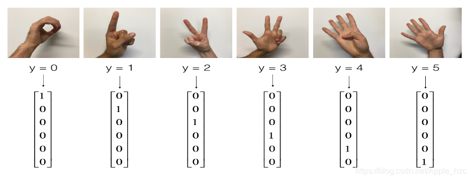
我们将通过tensorflow做出一个卷积模型，并通过它对数据集进行训练，提高其在测试集上的准确率。

以下是tensorflow model的步骤：

1. 创建createholders
2. 对参数进行初始化
3. 实现前向传播
4. 计算cost
5. 创建一个优化器对cost进行梯度下降算法

---

二、相关算法代码

import math
import numpy as np
import h5py
import matplotlib.pyplot as plt
import scipy
from PIL import Image
from scipy import ndimage
import tensorflow as tf
from tensorflow.python.framework import ops
from week1.cnn_utils import *
import os

os.environ['TF_CPP_MIN_LOG_LEVEL'] = '2'

np.random.seed(1)

X_train_orig, Y_train_orig, X_test_orig, Y_test_orig, classes = load_dataset()
# index = 15
# plt.imshow(X_train_orig[index])
# print("y = " + str(np.squeeze(Y_train_orig[:, index])))
# plt.show()
X_train = X_train_orig / 255.
X_test = X_test_orig / 255.
Y_train = convert_to_one_hot(Y_train_orig, 6).T
Y_test = convert_to_one_hot(Y_test_orig, 6).T
# print("number of training examples = " + str(X_train.shape[0]))
# print("number of test examples = " + str(X_test.shape[0]))
# print("X_train shape: " + str(X_train.shape))  # (1080, 64, 64, 3)
# print("Y_train shape: " + str(Y_train.shape))  # (1080, 6)
# print("X_test shape: " + str(X_test.shape))  # (120, 64, 64, 3)
# print("Y_test shape: " + str(Y_test.shape))  # (120, 6)
conv_layers = {}


def create_placeholders(n_H0, n_W0, n_C0, n_y):
    X = tf.placeholder('float', shape=[None, n_H0, n_W0, n_C0])
    Y = tf.placeholder('float', shape=[None, n_y])

    return X, Y


X, Y = create_placeholders(64, 64, 3, 6)


# print ("X = " + str(X))  # (?, 64, 64, 3)
# print ("Y = " + str(Y))  # (?, 6)


def initialize_parameters():
    tf.set_random_seed(1)

    W1 = tf.get_variable("W1", [4, 4, 3, 8], initializer=tf.contrib.layers.xavier_initializer(seed=0))
    W2 = tf.get_variable("W2", [2, 2, 8, 16], initializer=tf.contrib.layers.xavier_initializer(seed=0))

    parameters = {"W1": W1, "W2": W2}

    return parameters


# tf.reset_default_graph()
# with tf.Session() as sess_test:
#     parameters = initialize_parameters()
#     init = tf.global_variables_initializer()
#     sess_test.run(init)
#     print("W1 = " + str(parameters["W1"].eval()[1, 1, 1]))
#     print("W2 = " + str(parameters["W2"].eval()[1, 1, 1]))


def forward_propagation(X, parameters):
    W1 = parameters['W1']
    W2 = parameters['W2']

    Z1 = tf.nn.conv2d(X, W1, strides=[1, 1, 1, 1], padding='SAME')
    A1 = tf.nn.relu(Z1)
    P1 = tf.nn.max_pool(A1, ksize=[1, 8, 8, 1], strides=[1, 8, 8, 1], padding='SAME')
    Z2 = tf.nn.conv2d(P1, W2, strides=[1, 1, 1, 1], padding='SAME')
    A2 = tf.nn.relu(Z2)
    P2 = tf.nn.max_pool(A2, ksize=[1, 4, 4, 1], strides=[1, 4, 4, 1], padding='SAME')
    P2 = tf.contrib.layers.flatten(P2)
    Z3 = tf.contrib.layers.fully_connected(P2, 6, activation_fn=None)

    return Z3


# tf.reset_default_graph()
# with tf.Session() as sess:
#     np.random.seed(1)
#     X, Y = create_placeholders(64, 64, 3, 6)
#     parameters = initialize_parameters()
#     Z3 = forward_propagation(X, parameters)
#     init = tf.global_variables_initializer()
#     sess.run(init)
#     a = sess.run(Z3, {X: np.random.randn(2, 64, 64, 3), Y: np.random.randn(2, 6)})
#     print("Z3 = " + str(a))


def compute_cost(Z3, Y):
    cost = tf.reduce_mean(tf.nn.softmax_cross_entropy_with_logits_v2(logits=Z3, labels=Y))
    return cost


# tf.reset_default_graph()
# with tf.Session() as sess:
#     np.random.seed(1)
#     X, Y = create_placeholders(64, 64, 3, 6)
#     parameters = initialize_parameters()
#     Z3 = forward_propagation(X, parameters)
#     cost = compute_cost(Z3, Y)
#     init = tf.global_variables_initializer()
#     sess.run(init)
#     a = sess.run(cost, {X: np.random.randn(4, 64, 64, 3), Y: np.random.randn(4, 6)})
#     print("cost = " + str(a))


def model(X_train, Y_train, X_test, Y_test, learning_rate=0.009,
          num_epochs=100, minibatch_size=64, print_cost=True):
    '''
     Implements a three-layer ConvNet in Tensorflow:
        CONV2D -> RELU -> MAXPOOL -> CONV2D -> RELU -> MAXPOOL -> FLATTEN -> FULLYCONNECTED
    :param X_train: training set, of shape (None, 64, 64, 3)
    :param Y_train:test set, of shape (None, n_y = 6)
    :param X_test:training set, of shape (None, 64, 64, 3)
    :param Y_test:test set, of shape (None, n_y = 6)
    :param learning_rate:learning rate of the optimization
    :param num_epochs:number of epochs of the optimization loop
    :param minibatch_size:size of a minibatch
    :param print_cost:True to print the cost every 100 epochs
    :return:
    train_accuracy -- real number, accuracy on the train set (X_train)
    test_accuracy -- real number, testing accuracy on the test set (X_test)
    parameters -- parameters learnt by the model. They can then be used to predict.
    '''


    ops.reset_default_graph()
    tf.set_random_seed(1)
    seed = 3
    (m, n_H0, n_W0, n_C0) = X_train.shape
    n_y = Y_train.shape[1]
    costs = []

    X, Y = create_placeholders(n_H0, n_W0, n_C0, n_y)

    parameters = initialize_parameters()

    Z3 = forward_propagation(X, parameters)

    cost = compute_cost(Z3, Y)

    optimizer = tf.train.AdamOptimizer(learning_rate).minimize(cost)

    init = tf.global_variables_initializer()

    with tf.Session() as sess:
        sess.run(init)
        for epoch in range(num_epochs):
            minibatch_cost = 0.
            num_minibatches = int(m / minibatch_size)
            seed = seed + 1
            minibatches = random_mini_batches(X_train, Y_train, minibatch_size, seed)
            for minibatch in minibatches:
                (minibatch_X, minibatch_Y) = minibatch
                _, temp_cost = sess.run([optimizer, cost] , feed_dict={X: minibatch_X, Y: minibatch_Y})

                minibatch_cost += temp_cost / num_minibatches

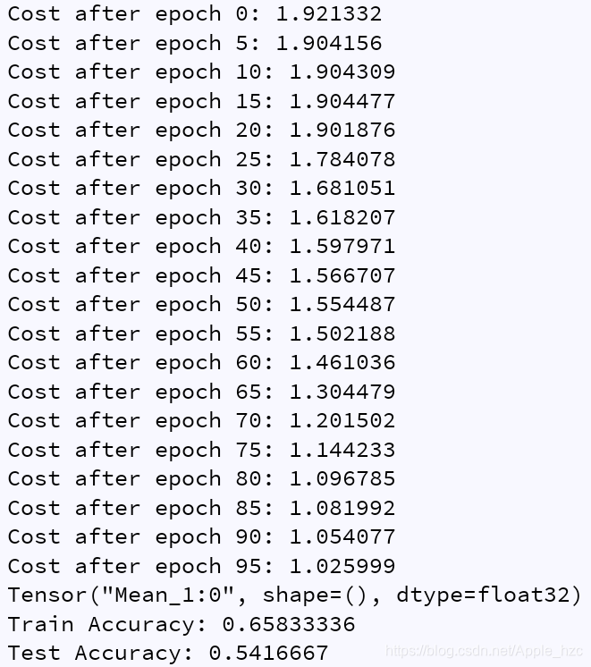
            if print_cost == True and epoch % 5 == 0:
                print("Cost after epoch %i: %f" % (epoch, minibatch_cost))
            if print_cost == True and epoch % 1 == 0:
                costs.append(minibatch_cost)

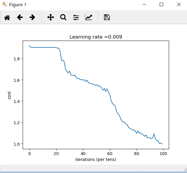
        plt.plot(np.squeeze(costs))
        plt.ylabel('cost')
        plt.xlabel('iterations (per tens)')
        plt.title("Learning rate =" + str(learning_rate))
        plt.show()

        predict_op = tf.argmax(Z3, 1)
        correct_prediction = tf.equal(predict_op, tf.argmax(Y, 1))

        accuracy = tf.reduce_mean(tf.cast(correct_prediction, "float"))
        print(accuracy)
        train_accuracy = accuracy.eval({X: X_train, Y: Y_train})
        test_accuracy = accuracy.eval({X: X_test, Y: Y_test})
        print("Train Accuracy:", train_accuracy)
        print("Test Accuracy:", test_accuracy)

        return train_accuracy, test_accuracy, parameters


_, _, parameters = model(X_train, Y_train, X_test, Y_test)

---

三、总结

到目前为止，我们通过tensorflow建立了一个识别手语的模型。如果想进一步提高准确性，可以尝试将超参数调优或者使用正则化等相关方法。