一、deeplearning-assignment
在本次任务中,我们将学习用numpy实现卷积(CONV)层和池化(POOL)层,由于大多数深度学习工程师不需要关注反向传递的细节,而且卷积网络的反向传递很复杂,所以在本次作业中只讨论关于前向传播的处理细节。
用 python 来实现每个函数,在下次任务用 TensorFlow 中等价的函数构造如下模型:

对于每个前向传播,都有相应的反向传播。因此,每一步前向传播,都会存储一些参数在缓存中。这些参数用于计算反向传播中的梯度。
卷积神经网络
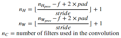
尽管编程框架使得卷积操作易于实现,但它仍然是深度学习中最难理解的概念之一。卷积层将输入转换为不同尺寸的输出:

在实现卷积神经网络之前,首先要实现两个辅助函数:一个用于零填充,另一个用于卷积计算。
零填充
指的是在图像的边缘填充一系列的零点。


上图中,将一个图像(三个通道对应三个RGB值)的每一层RGB矩阵进行padding为2的零填充。
零填充的主要好处如下:
-
它允许你在不缩小宽度和高度的同时使用CONV层. 这对构建更深层次的网络非常重要, 否则网络越深,宽度/高度越小. 一个重要的特殊案例是 "same" convolution, 它在经历一层卷积后宽度/高度维持不变.
-
它会在图像的边界保留更多的信息. 如果没有填充,下一层的极少数值会受到边缘像素的影响。
卷积计算

将过滤器对应于Image中对应的位置,进行乘法运算后将累加和输出到新矩阵对应的位置,然后通过步长平移相应的位置重复之前的步骤,直到输出矩阵计算完毕。
卷积神经网络的前向传播
在正向传递中,将对输入采用多种过滤器进行卷积。每个“卷积”输出一个二维矩阵。最后叠加二维矩阵获得3D volume。

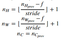
池化层
池化层会降低输入的高度和宽度。它有助于减少计算量,主要有两种类型的池化,如下图所示:

池化层中相关参数的计算:
二、相关算法代码
import numpy as np
import h5py
import matplotlib.pyplot as plt

plt.rcParams['figure.figsize'] = (5.0, 4.0)  # set default size of plots
plt.rcParams['image.interpolation'] = 'nearest'
plt.rcParams['image.cmap'] = 'gray'

np.random.seed(1)


def zero_pad(X, pad):
    X_pad = np.pad(X, ((0, 0), (pad, pad), (pad, pad), (0, 0)), 'constant')
    return X_pad


# np.random.seed(1)
# x = np.random.randn(4, 3, 3, 2)
# x_pad = zero_pad(x, 2)
# print("x.shape =", x.shape)
# print("x_pad.shape =", x_pad.shape)
# print("x[1,1] =", x[1, 1])
# print("x_pad[1,1] =", x_pad[1, 1])
# fig, axarr = plt.subplots(1, 2)
# axarr[0].set_title('x')
# axarr[0].imshow(x[0, :, :, 0])
# axarr[1].set_title('x_pad')
# axarr[1].imshow(x_pad[0, :, :, 0])
# plt.show()


def conv_single_step(a_slice_prev, W, b):
    s = a_slice_prev * W
    Z = np.sum(s)
    Z = float(Z + b)
    return Z


# np.random.seed(1)
# a_slice_prev = np.random.randn(4, 4, 3)
# W = np.random.randn(4, 4, 3)
# b = np.random.randn(1, 1, 1)
# Z = conv_single_step(a_slice_prev, W, b)
# print("Z =", Z)


def conv_forward(A_prev, W, b, hparameters):
    (m, n_H_prev, n_W_prev, n_C_prev) = A_prev.shape
    (f, f, n_C_prev, n_C) = W.shape

    stride = hparameters['stride']
    pad = hparameters['pad']

    n_H = int((n_H_prev - f + 2 * pad) / stride + 1)
    n_W = int((n_W_prev - f + 2 * pad) / stride + 1)

    Z = np.zeros((m, n_H, n_W, n_C))

    A_prev_pad = zero_pad(A_prev, pad)

    for i in range(m):
        a_prev_pad = A_prev_pad[i, :, :, :]
        for h in range(n_H):
            for w in range(n_W):
                for c in range(n_C):
                    vert_start = h * stride
                    vert_end = vert_start + f
                    horiz_start = w * stride
                    horiz_end = horiz_start + f

                    a_slice_prev = a_prev_pad[vert_start: vert_end, horiz_start: horiz_end, :]

                    Z[i, h, w, c] = conv_single_step(a_slice_prev, W[:, :, :, c], b[:, :, :, c])

    assert (Z.shape == (m, n_H, n_W, n_C))

    cache = (A_prev, W, b, hparameters)

    return Z, cache


# np.random.seed(1)
# A_prev = np.random.randn(10, 4, 4, 3)
# W = np.random.randn(2, 2, 3, 8)
# b = np.random.randn(1, 1, 1, 8)
# hparameters = {"pad": 2,
#                "stride": 2}
# Z, cache_conv = conv_forward(A_prev, W, b, hparameters)
# print("Z.shape = ", Z.shape)
# print("Z's mean = ", np.mean(Z))
# print("Z[3,2,1] = ", Z[3, 2, 1])
# print("cache_conv[0][1][2][3] =", cache_conv[0][1][2][3])


def pool_forward(A_prev, hparameters, mode='max'):
    (m, n_H_prev, n_W_prev, n_C_prev) = A_prev.shape
    f = hparameters['f']
    stride = hparameters['stride']

    n_H = int(1 + (n_H_prev - f) / stride)
    n_W = int(1 + (n_W_prev - f) / stride)
    n_C = n_C_prev

    A = np.zeros((m, n_H, n_W, n_C))

    for i in range(m):
        for h in range(n_H):
            for w in range(n_W):
                for c in range(n_C):
                    vert_start = h * stride
                    vert_end = vert_start + stride
                    horiz_start = w * stride
                    horiz_end = horiz_start + stride

                    a_prev_slice = A_prev[i, vert_start:vert_end, horiz_start:horiz_end, c]

                    if mode == "max":
                        A[i, h, w, c] = np.max(a_prev_slice)
                    elif mode == "average":
                        A[i, h, w, c] = np.mean(a_prev_slice)

    cache = (A_prev, hparameters)
    assert (A.shape == (m, n_H, n_W, n_C))

    return A, cache


np.random.seed(1)
A_prev = np.random.randn(2, 4, 4, 3)
hparameters = {"stride": 2, "f": 3}
A, cache = pool_forward(A_prev, hparameters)
print("mode = max")
print("A =", A)
print()
A, cache = pool_forward(A_prev, hparameters, mode="average")
print("mode = average")
print("A =", A)
三、总结
在前面的学习中,我们知道了怎样通过numpy建立辅助函数来理解卷积神经网络背后的机制,包括零填充、卷积计算以及池化层等相关的操作。不过今天大多数实际应用的深度学习都会使用编程框架,有很多内置函数可以简单地调用,在下次的work中,我们将学习运用tensorflow框架来实现卷积神经网络。