版权声明:本文为博主原创文章,未经博主允许不得转载。 https://blog.csdn.net/Apple_hzc/article/details/83049371
一、deeplearning-assignment
在本周作业的编程中,主要通过构建两层神经网络和L层神经网络对catvnoncat.h5数据集进行学习和预测,并得到对test数据集的预测准确度以及判断一张图片是否为猫。
在前面的作业中,我们通过逻辑回归模型对该数据集进行了学习和预测,准确度为70%(可以翻看之前的博客和参阅相关代码结果),今天主要构建深层神经网络对数据集进行学习。
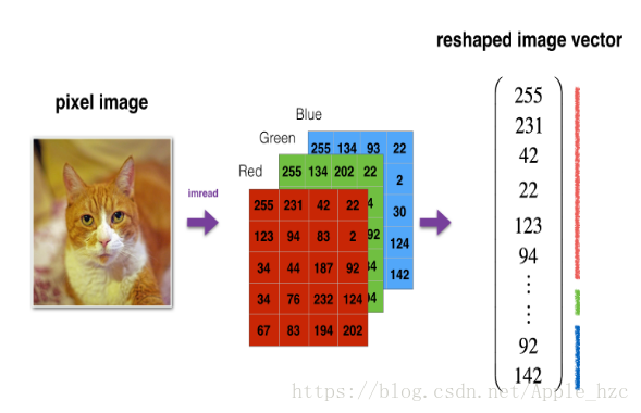
由上图可以看出,输入X中的每一列是一个(64 * 64 * 3,1)的列向量,即(12288,1)。
2层神经网络结构图:
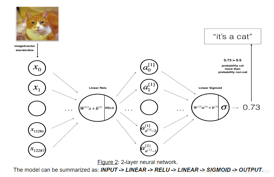
从图中我们可以看到,首先喂入一个X,通过线性运算得到Z1,接着通过非线性激活函数RELU得到A1,并作为输入赋给第二层,同样通过线性运算得到Z2,最后通过sigmoid函数得到预测值A2,完成前向传播过程。
L层神经网络结构图:

与2层神经网络类似,L层神经网络的前向传播是进行L - 1次(线性运算+RELU),最后通过sigmoid得到预测值。
下面看看代码。
二、相关算法代码
import time
import numpy as np
import h5py
import matplotlib.pyplot as plt
import scipy
from PIL import Image
from scipy import ndimage
from dnn_app_utils_v2 import *
plt.rcParams['figure.figsize'] = (5.0, 4.0) # set default size of plots
plt.rcParams['image.interpolation'] = 'nearest'
plt.rcParams['image.cmap'] = 'gray'
np.random.seed(1)
train_x_orig, train_y, test_x_orig, test_y, classes = load_data()
# index = 7
# plt.imshow(train_x_orig[index])
# plt.show()
# print("y = " + str(train_y[0, index]) + ". It's a " +
# classes[train_y[0, index]].decode("utf-8") + " picture.")
# m_train = train_x_orig.shape[0]
num_px = train_x_orig.shape[1]
# m_test = test_x_orig.shape[0]
# print("Number of training examples: " + str(m_train))
# print("Number of testing examples: " + str(m_test))
# print("Each image is of size: (" + str(num_px) + ", " + str(num_px) + ", 3)")
# print("train_x_orig shape: " + str(train_x_orig.shape))
# print("train_y shape: " + str(train_y.shape))
# print("test_x_orig shape: " + str(test_x_orig.shape))
# print("test_y shape: " + str(test_y.shape))
# Reshape the training and test examples
train_x_flatten = train_x_orig.reshape(train_x_orig.shape[0],
-1).T # The "-1" makes reshape flatten the remaining dimensions
test_x_flatten = test_x_orig.reshape(test_x_orig.shape[0], -1).T
# Standardize data to have feature values between 0 and 1.
train_x = train_x_flatten / 255.
test_x = test_x_flatten / 255.
# print("train_x's shape: " + str(train_x.shape))
# print("test_x's shape: " + str(test_x.shape))
n_x = 12288 # num_px * num_px * 3
n_h = 7
n_y = 1
layers_dims = (n_x, n_h, n_y)
def two_layer_model(X, Y, layers_dims, learning_rate=0.0075, num_iterations=3000, print_cost=False):
"""
:param X:input data, of shape (n_x, number of examples)
:param Y:true "label" vector (containing 0 if cat, 1 if non-cat), of shape (1, number of examples)
:param layers_dims:dimensions of the layers (n_x, n_h, n_y)
:param learning_rate:learning rate of the gradient descent update rule
:param num_iterations:number of iterations of the optimization loop
:param print_cost:If set to True, this will print the cost every 100 iterations
:return:parameters -- a dictionary containing W1, W2, b1, and b2
"""
np.random.seed(1)
grads = {}
costs = [] # to keep track of the cost
m = X.shape[1] # number of examples
(n_x, n_h, n_y) = layers_dims
parameters = initialize_parameters(n_x, n_h, n_y)
W1 = parameters["W1"]
b1 = parameters["b1"]
W2 = parameters["W2"]
b2 = parameters["b2"]
for i in range(0, num_iterations):
# Forward propagation: LINEAR -> RELU -> LINEAR -> SIGMOID. Inputs: "X, W1, b1".
# Output: "A1, cache1, A2, cache2".
A1, cache1 = linear_activation_forward(X, W1, b1, "relu")
A2, cache2 = linear_activation_forward(A1, W2, b2, "sigmoid")
# Compute cost
cost = compute_cost(A2, Y)
# Initializing backward propagation
dA2 = - (np.divide(Y, A2) - np.divide(1 - Y, 1 - A2))
# Backward propagation. Inputs: "dA2, cache2, cache1".
# Outputs: "dA1, dW2, db2; also dA0 (not used), dW1, db1".
dA1, dW2, db2 = linear_activation_backward(dA2, cache2, 'sigmoid')
dA0, dW1, db1 = linear_activation_backward(dA1, cache1, 'relu')
grads['dW1'] = dW1
grads['db1'] = db1
grads['dW2'] = dW2
grads['db2'] = db2
# Update parameters.
parameters = update_parameters(parameters, grads, learning_rate)
W1 = parameters["W1"]
b1 = parameters["b1"]
W2 = parameters["W2"]
b2 = parameters["b2"]
if print_cost and i % 100 == 0:
print("Cost after iteration {}: {}".format(i, np.squeeze(cost)))
if print_cost and i % 100 == 0:
costs.append(cost)
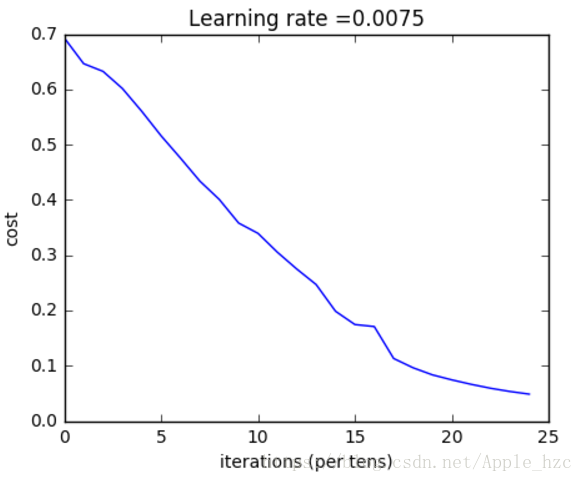
plt.plot(np.squeeze(costs))
plt.ylabel('cost')
plt.xlabel('iterations (per tens)')
plt.title("Learning rate =" + str(learning_rate))
plt.show()
return parameters
# parameters = two_layer_model(train_x, train_y, layers_dims=(n_x, n_h, n_y), num_iterations=2000, print_cost=True)
# predictions_train = predict(train_x, train_y, parameters)
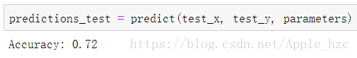
# predictions_test = predict(test_x, test_y, parameters)
layers_dims = [12288, 20, 7, 5, 1] # 5-layer model
def L_layer_model(X, Y, layers_dims, learning_rate=0.0075, num_iterations=3000, print_cost=False):
"""
:param X:data, numpy array of shape (number of examples, num_px * num_px * 3)
:param Y:data, numpy array of shape (number of examples, num_px * num_px * 3)
:param layers_dims:list containing the input size and each layer size, of length (number of layers + 1).
:param learning_rate:learning rate of the gradient descent update rule
:param num_iterations:number of iterations of the optimization loop
:param print_cost:if True, it prints the cost every 100 steps
:return:parameters -- parameters learnt by the model. They can then be used to predict.
"""
np.random.seed(1)
costs = []
parameters = initialize_parameters_deep(layers_dims)
for i in range(0, num_iterations):
# Forward propagation: [LINEAR -> RELU]*(L-1) -> LINEAR -> SIGMOID.
AL, caches = L_model_forward(X, parameters)
# Compute cost.
cost = compute_cost(AL, Y)
# Backward propagation.
grads = L_model_backward(AL, Y, caches)
# Update parameters.
parameters = update_parameters(parameters, grads, learning_rate)
if print_cost and i % 100 == 0:
print("Cost after iteration %i: %f" % (i, cost))
if print_cost and i % 100 == 0:
costs.append(cost)
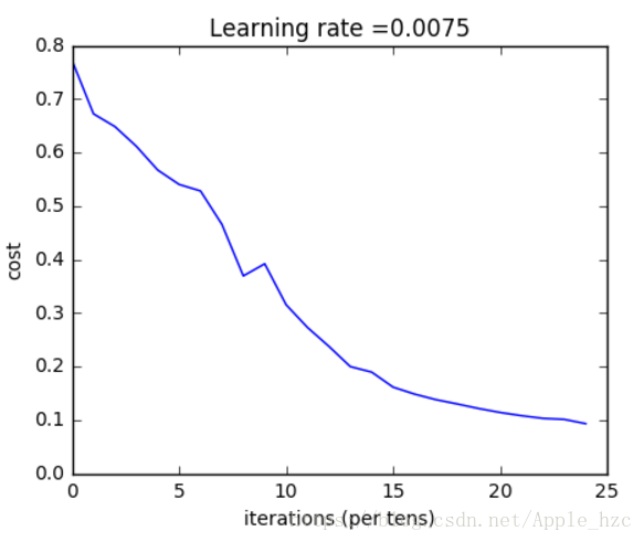
plt.plot(np.squeeze(costs))
plt.ylabel('cost')
plt.xlabel('iterations (per tens)')
plt.title("Learning rate =" + str(learning_rate))
plt.show()
return parameters
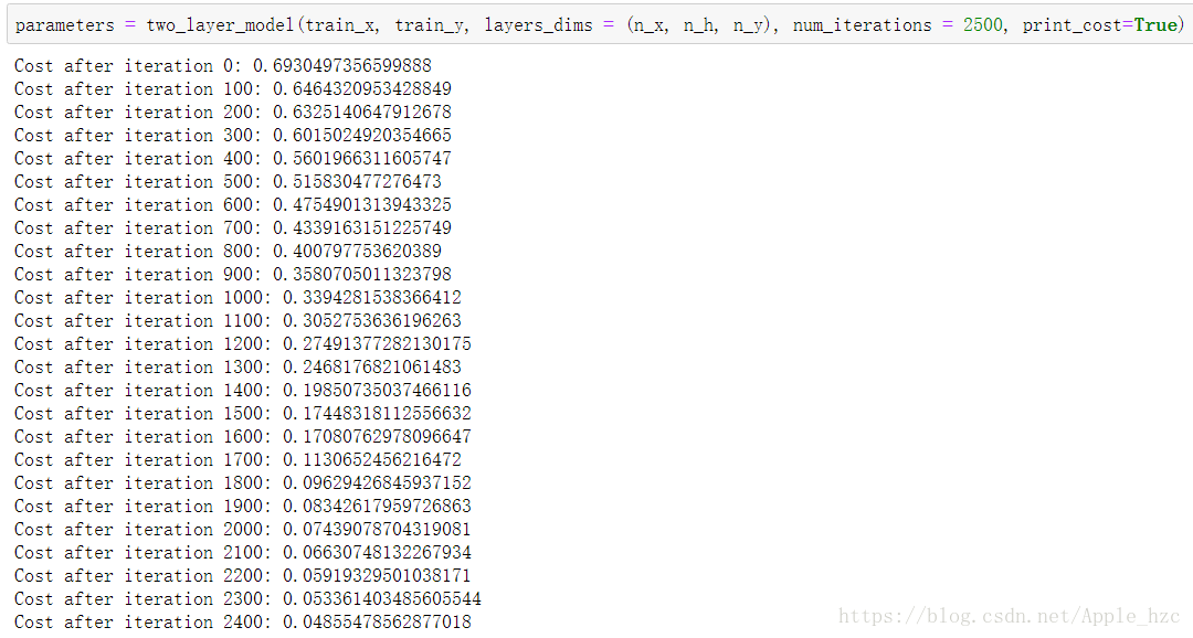
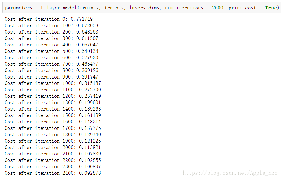
parameters = L_layer_model(train_x, train_y, layers_dims, num_iterations=2500, print_cost=True)
# pred_train = predict(train_x, train_y, parameters)
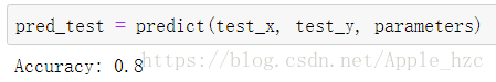
# pred_test = predict(test_x, test_y, parameters)
my_image = "la_defense.jpg" # change this to the name of your image file
my_label_y = [0] # the true class of your image (1 -> cat, 0 -> non-cat)
fname = "e:/code/Python/DeepLearning/Neural networks and deep learning/week2/images/" + my_image
image = np.array(ndimage.imread(fname, flatten=False, mode='RGB'))
my_image = scipy.misc.imresize(image, size=(num_px, num_px)).reshape((num_px * num_px * 3, 1))
my_predicted_image = predict(my_image, my_label_y, parameters)
plt.imshow(image)
plt.show()
print("y = " + str(np.squeeze(my_predicted_image)) + ", your L-layer model predicts a \"" + classes[
int(np.squeeze(my_predicted_image)), ].decode("utf-8") + "\" picture.")
最后通过随机的一张图片,利用以上神经网络进行判断(代码的最后几行):
得出结论:

三、总结
通过本周作业的练习,对深层神经网络的正向传播和反向传播有了更深刻的理解,知道如何通过代码来实现和构建网络,并利用网络对数据集进行学习和预测。
总结构建深层神经网络步骤:
初始化工作
- 定义一个2层的神经网络
- L-layer Neural Network:定义一个
层网络
- initialize_parameters_deep(layer_dims) --> parameters(parameters是一个字典,包含每一层的权重和偏差,例如parameters['W1']则可以得到第一层的权重)
前向传播
- linear_forward(A, W, b) --> Z, cache
- (cache=(A, W, b))
- linear_activation_forward(A_prev, W, b, activation) --> A
- cache=(linear_cache, activation_cache),其中linear_cache=(A_pre, W, b),activation_cache=z
- L_model_forward(X, parameters) --> AL,caches (AL表示最后一层的计算值, caches存储的是
损失函数
compute_cost(AL, Y) --> cost
反向传播
- linear_backward(dZ, cache) --> dA_prev, dW, db 其中的输入值 cache=(A, W, b)
- linear_activation_backward(dA, cache, activation) --> dA_prev, dW, db
- cache=(linear_cache, activation_cache),其中linear_cache=(A,W,b),activation_cache=z
- L_model_backward(AL, Y, caches)-->grads(grads是一个字典,包含grads["dWl"],grads["dbl"],grads["dAl"],其中l=1,2...L)
- update_parameters(parameters, grads, learning_rate) --> parameters(parameters表示更新后的所有权重,可以通过parameters['W1']获得第一层的权重。)