聚类算法(2)--Mean Shift

Mean shift 算法是基于核密度估计的爬山算法，可用于聚类、图像分割、跟踪等，因为最近搞一个项目，涉及到这个算法的图像聚类实现，因此这里做下笔记。

mean shift 算法理论

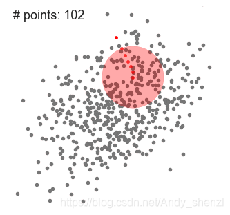
Mean-shift（即：均值迁移）的基本思想：在数据集中选定一个点，然后以这个点为圆心，r为半径，画一个圆(二维下是圆)，求出这个点到所有点的向量的平均值，而圆心与向量均值的和为新的圆心，然后迭代此过程，直到满足一点的条件结束。(Fukunage在1975年提出)

Mean-Shift是一种基于滑动窗口的聚类算法。也可以说它是一种基于质心的算法，这意思是它是通过计算滑动窗口中的均值来更新中心点的候选框，以此达到找到每个簇中心点的目的。然后在剩下的处理阶段中，对这些候选窗口进行滤波以消除近似或重复的窗口，找到最终的中心点及其对应的簇。

整体的图例如下：

分步骤演示：

步骤1：在指定的区域内计算偏移均值(如下图的黄色的圈)

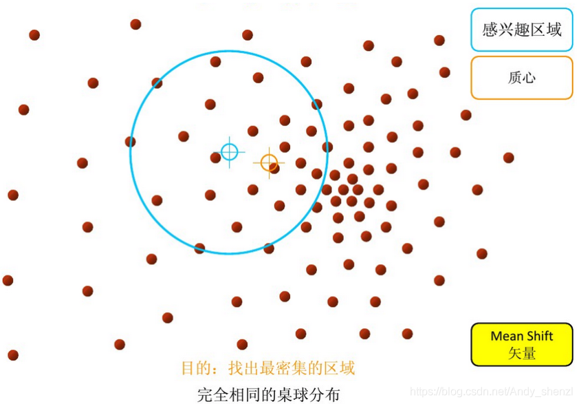
步骤2：移动该点到偏移均值点处

步骤3：重复上述的过程(计算新的偏移均值，移动)

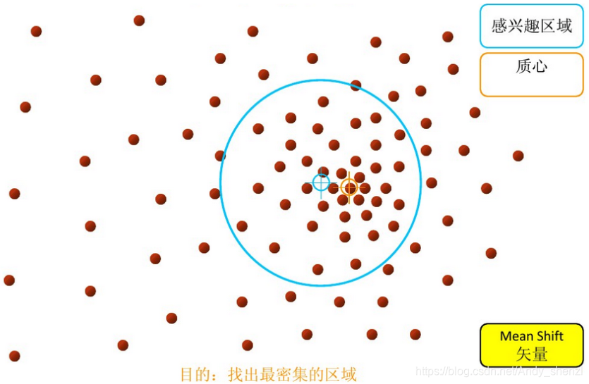
我们再用一个比较直观的实例看一下：

基本的Mean Shift向量形式

sklearn参数

[class sklearn.cluster.MeanShift]

bandwidth=None： float，高斯核函数的半径(或带宽)，如果没有给定，则使用sklearn.cluster.estimate_bandwidth 自动估计带宽；

seeds=None： array, shape=[n_samples, n_features]，我理解的 seeds 是初始化的质心，如果为 None 并且 bin_seeding=True，就用 clustering.get_bin_seeds 计算得到；

bin_seeding=False： boolean，在没有设置 seeds 时起作用，如果 bin_seeding=True，就用 clustering.get_bin_seeds 计算得到质心，如果 bin_seeding=False，则设置所有点为质心；

min_bin_freq=1： int，clustering.get_bin_seeds 的参数，设置的最少质心个数；
以上三个参数要结合起来理解；

cluster_all=True： boolean，如果为 True，所有的点都会被聚类，包括不在任何核内的孤立点，其会选择一个离自己最近的核；如果为 False，孤立点的类标签为 -1；

n_jobs=1： int，多线程；
                    -1：使用所有的cpu；
                    1：不使用多线程；
                  -2：如果 n_jobs<0，(n_cpus + 1 + n_jobs)个cpu被使用，所以 n_jobs=-2 时，所有的cpu中只有一块不被使用；

主要属性

cluster_centers_ : 数组类型。计算出的聚类中心的坐标。

labels_ :数组类型。每个数据点的分类标签。

python—sklearn实例演示

我们运用K-means里面的一个数据样本：

import numpy as np
cluster1 = np.random.uniform(0.5, 1.5, (2, 10))
cluster2 = np.random.uniform(3.5, 4.5, (2, 10))
X = np.hstack((cluster1, cluster2)).T#合并数据
plt.figure()
plt.axis([0, 5, 0, 5])
plt.grid(True)
plt.plot(X[:,0],X[:,1],'k.')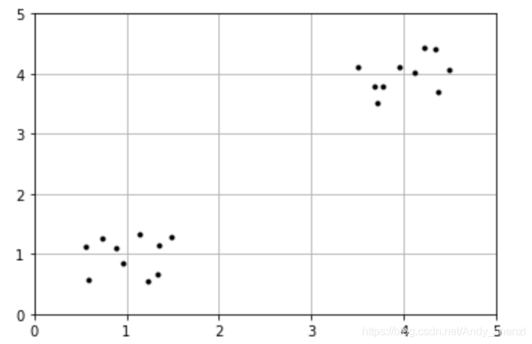

导入相关包

from sklearn.cluster import MeanShift, estimate_bandwidth

bandwidth1 = estimate_bandwidth(X, quantile=0.2)

ms = MeanShift(bandwidth=bandwidth, bin_seeding=True)
ms.fit(X)
labels = ms.labels_
cluster_centers = ms.cluster_centers_

labels_unique = np.unique(labels)
n_clusters_ = len(labels_unique)

print("number of estimated clusters : %d" % n_clusters_)

number of estimated clusters : 2

import matplotlib.pyplot as plt
from itertools import cycle

plt.figure(1)
plt.clf()

colors = cycle('bgrcmykbgrcmykbgrcmykbgrcmyk')
for k, col in zip(range(n_clusters_), colors):
    my_members = labels == k
    cluster_center = cluster_centers[k]
    plt.plot(X[my_members, 0], X[my_members, 1], col + '.')
    plt.plot(cluster_center[0], cluster_center[1], 'o', markerfacecolor=col,
             markeredgecolor='k', markersize=14)
plt.title('Estimated number of clusters: %d' % n_clusters_)
plt.show()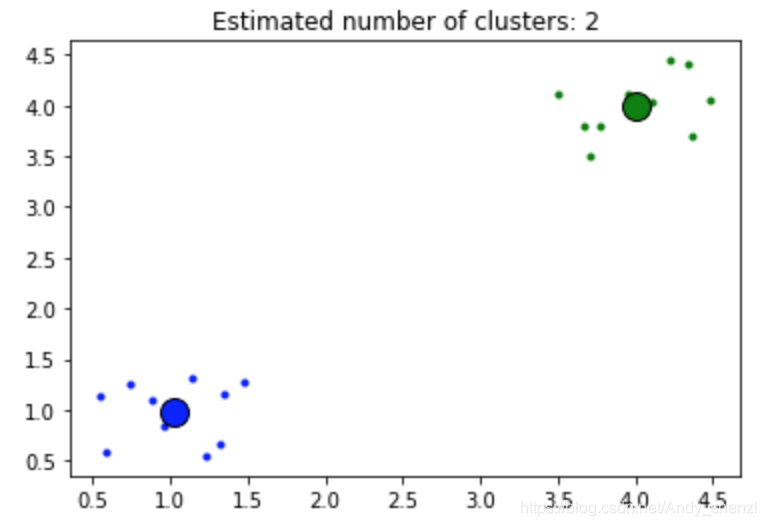

PS：

bandwidth=None： float，高斯核函数的半径(或带宽)，如果没有给定，则使用sklearn.cluster.estimate_bandwidth 自动估计带宽

我们上面就是运用了sklearn.cluster.estimate_bandwidth计算了bandwidth

对于bandwidth我们简单解释下

estimate_bandwidth(X, quantile=0.3, n_samples=None, random_state=0, n_jobs=None)

X : array-like, shape=[n_samples, n_features]

Input points.

quantile : float, default 0.3

should be between [0, 1] 0.5 means that the median of all pairwise distances is used.

n_samples : int, optional

The number of samples to use. If not given, all samples are used.

random_state : int, RandomState instance or None (default)

The generator used to randomly select the samples from input points for bandwidth estimation. Use an int to make the randomness deterministic. See Glossary.

n_jobs : int or None, optional (default=None)

The number of parallel jobs to run for neighbors search. None means 1 unless in a joblib.parallel_backend context. -1 means using all processors. See Glossary for more details.

举个例子对quantile的影响来看一下：

import numpy as np
X0 = np.array([7, 5, 7, 3, 4, 1, 0, 2, 8, 6, 5, 3])
X1 = np.array([5, 7, 7, 3, 6, 4, 0, 2, 7, 8, 5, 7])
X00=np.array(list(zip(X0, X1))).reshape(len(X0), 2)#组合数据
import matplotlib.pyplot as plt 
plt.figure()
plt.scatter(X00[:, 0], X00[:, 1],c='b')#原始数据散点图

from sklearn.cluster import MeanShift, estimate_bandwidth
for a in list(range(2,10,1)):
    b=a/10
    bandwidth = estimate_bandwidth(X00, quantile=b)
    ms = MeanShift(bandwidth=bandwidth, bin_seeding=True)
    ms.fit(X00)
    labels = ms.labels_
    cluster_centers = ms.cluster_centers_

    labels_unique = np.unique(labels)
    n_clusters_ = len(labels_unique)

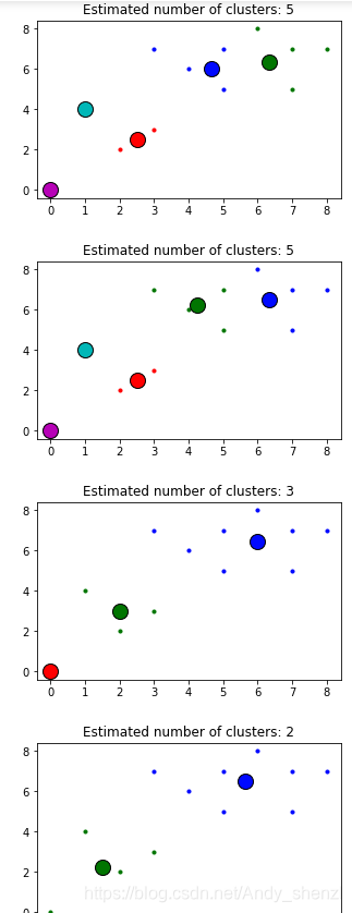
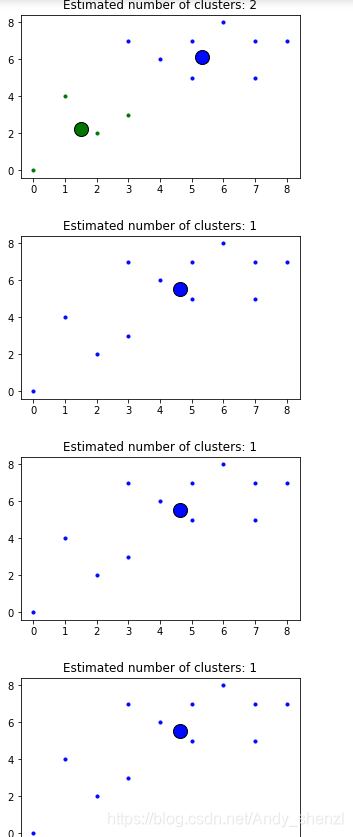
    print("number of estimated clusters : %d" % n_clusters_)

number of estimated clusters : 5
number of estimated clusters : 5
number of estimated clusters : 3
number of estimated clusters : 2
number of estimated clusters : 2
number of estimated clusters : 1
number of estimated clusters : 1
number of estimated clusters : 1

我们可以看到随着 quantile的增大，聚类的数量随之减少。


for a in list(range(2,10,1)):
    b=a/10
    
    bandwidth = estimate_bandwidth(X00, quantile=b)
    ms = MeanShift(bandwidth=bandwidth, bin_seeding=True)
    ms.fit(X00)
    labels = ms.labels_
    cluster_centers = ms.cluster_centers_

    labels_unique = np.unique(labels)
    n_clusters_ = len(labels_unique)

    plt.figure(figsize=(16, 16))
    colors = cycle('bgrcmykbgrcmykbgrcmykbgrcmyk')
    for k, col in zip(range(n_clusters_), colors):
        my_members = labels == k
        cluster_center = cluster_centers[k]
        plt.plot(X00[my_members, 0], X00[my_members, 1], col + '.')
        plt.plot(cluster_center[0], cluster_center[1], 'o', markerfacecolor=col,
             markeredgecolor='k', markersize=14)
    plt.title('Estimated number of clusters: %d' % n_clusters_)
    plt.show()
plt.savefig('test1')