HelloDNN，多层感知机MLP学习笔记

前言
学那个技术第一步都是helloworld，AI也是一样，我们来吧

1、从感知机说起

这是一个3输入1输出的感知机模型

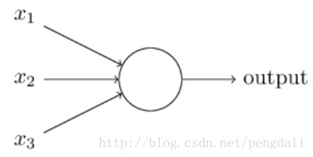
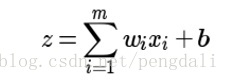
输入输出之间学到一个线性关系

然后一个神经元激活函数

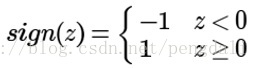
但这类模型无法学习比较复杂的非线性模型，且只能做2元分类

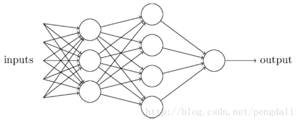
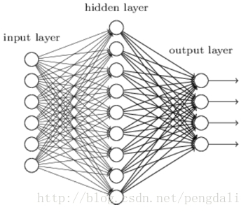
2、引入多层感知机神经网络

MLP在对感知机进行的改进主要有3点
2.1 隐藏层
主要为了加强表达能力，层数越多自然表达能力高，当然参数也线性增多，训练时、前向时计算量也越大，所以找到一个合适需求的

2.2 多输出
输出层的神经元不止1个，根据需求设计出多个输出，一般的分类回归都是有多个输出的吧

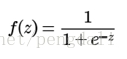
2.3 激活函数的扩展
神经网络中一般使用的sigmoid，softmax，relu，tanx等等，比如一般会用softmax解决分类问题，隐层为了防止梯度消失会选用relu，回归问题会用sigmoid，如：

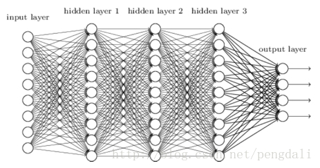
好了，我们最后看个一般的MLP模型，每层之间的节点做全连接，参数量爆多，难怪要用显卡

3、代码中学习MLP

这里使用tensorflow来做这个HelloWorld（mnist）
因为是HelloWorld所以用一个最简单的1个全连接层10个节点的结构
3.1 构建模型

    def inference(self):
        self.input = tf.placeholder(tf.float32, [None, 784])         #输入28*28的图
        self.label = tf.placeholder(tf.float32, [None, 10])          #正确的分类标签
        with tf.variable_scope('model'):
            w = tf.Variable(tf.truncated_normal([784,10],stddev=0.1))            #权重参数
            b = tf.Variable(tf.zeros([10]))         #偏置参数
            y = tf.nn.softmax(tf.matmul(self.input, w) + b)          # 10个分类输出（0-9数字）

        with tf.variable_scope('optimize'):
            cross_entropy = tf.reduce_mean(-tf.reduce_sum(self.label * tf.log(y), reduction_indices=[1]))       #使用交叉熵获得损失函数
            self.train_step = tf.train.GradientDescentOptimizer(0.5).minimize(cross_entropy)         #使用梯度下降法最小化损失函数

        with tf.variable_scope('accuracy'):
            correct_prediction = tf.equal(tf.argmax(y, 1), tf.argmax(self.label, 1))        #预测值是否正确
            self.accuracy = tf.reduce_mean(tf.cast(correct_prediction, tf.float32))         #求正确率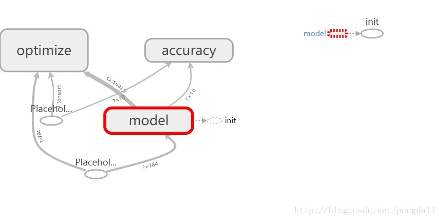

这里分成3个部分
1)model，它简单到只有输入、输出层，输入mnist数据(28*28)，然后直接输出10分类
2)optimize，它主要是为了训练这个模型，后面详细分析下
3)accuracy，它是为了验证这个模型拟合的好不好

3.2 优化过程

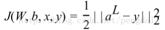
我们需要一个损失函数来度量训练样本的输出损失，对这个损失函数进行优化求最小的极值，一般是通过梯度下降发来进行一步一步循环迭代来完成的，所以我们要训练那么多次

拿到前向结果带入到损失函数中，损失函数有非常多，最常见的是均方差来度量损失，对每个样本期望最小化这个式子

然后在使用梯度下降法求解每一层的w,b，下面把前面说的结合代码的再过一遍

1) 先拿到前向结果y,这里比如预测出的10个分类值是：
[[ 0.02168657 0.02897528 0.11036823 0.06726296 0.05238539 0.05396876
0.19831 0.06922533 0.3276386 0.0701789 ]]

2) 对y进行求导tf.log(y)，这里得到
[[-3.83106184 -3.54131222 -2.203933 -2.69914556 -2.94912744 -2.91934991
-1.61792386 -2.67038846 -1.11584413 -2.65670753]]

3) 训练标签的数据是one_hot编码的，拿他和求导值做乘法self.label * tf.log(y)，比如得到
[[ 0. 0. 0. 0. 0. 0. 0.
0. -1.11584413 0. ]]

4) 整理下，在y轴上求和-tf.reduce_sum(self.label * tf.log(y), reduction_indices=[1])
[ 1.11584413 ]

5)我们一批数据有100条，上面说的是1条数据，接下来就是对它们进行求平均，把上面的步骤合在一起就是求交叉熵

tf.reduce_mean(-tf.reduce_sum(self.label * tf.log(y), reduction_indices=[1]))

6) 最后我们再使用梯度下降优化器做损失函数，学习率参数0.5，这个可以自己调调看
业界使用最多的是mini-Batch的梯度下降法，不过这个要看训练样本而定

tf.train.GradientDescentOptimizer(0.5).minimize(cross_entropy)

3.3 训练与验证

    def train(self):
        with tf.Session() as sess:
            sess.run(tf.global_variables_initializer())
            for i in range(1000):               #训练1000轮，每次100条数据
                batch_data, batch_label = self.mnist.train.next_batch(100)
                sess.run(self.train_step,{self.input:batch_data, self.label:batch_label})
            print('accuracy : %f' % sess.run(self.accuracy,{self.input: self.mnist.test.images, self.label: self.mnist.test.labels}))

分为3个步骤
1)先对变量进行初始化
2)循环训练
3)进行结果验证（使用test数据集）
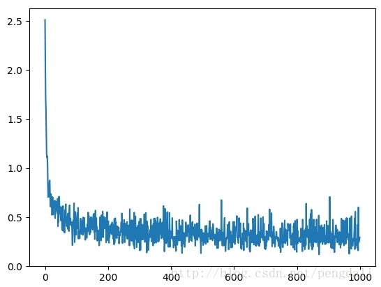
这个只训练了1000步的结果：
accuracy : 0.916000
这是loss的变化

3.4 代码

需要自己下载mnist数据库，放在MNIST_data目录下

import tensorflow as tf
from tensorflow.examples.tutorials.mnist import input_data

class hello_world:
    def __init__(self):
        self.mnist = input_data.read_data_sets("MNIST_data/", one_hot=True)

    def inference(self):
        self.input = tf.placeholder(tf.float32, [None, 784])         #输入28*28的图
        self.label = tf.placeholder(tf.float32, [None, 10])          #正确的分类标签
        with tf.variable_scope('model'):
            w = tf.Variable(tf.truncated_normal([784,10],stddev=0.1))            #权重参数
            b = tf.Variable(tf.zeros([10]))         #偏置参数
            y = tf.nn.softmax(tf.matmul(self.input, w) + b)          # 10个分类输出（0-9数字）

        with tf.variable_scope('optimize'):
            cross_entropy = tf.reduce_mean(-tf.reduce_sum(self.label * tf.log(y), reduction_indices=[1]))       #使用交叉熵获得损失函数
            self.train_step = tf.train.GradientDescentOptimizer(0.5).minimize(cross_entropy)         #使用梯度下降法最小化损失函数

        with tf.variable_scope('accuracy'):
            correct_prediction = tf.equal(tf.argmax(y, 1), tf.argmax(self.label, 1))        #预测值是否正确
            self.accuracy = tf.reduce_mean(tf.cast(correct_prediction, tf.float32))         #求正确率

    def train(self):
        with tf.Session() as sess:
            sess.run(tf.global_variables_initializer())
            for i in range(1000):               #训练1000轮，每次100条数据
                batch_data, batch_label = self.mnist.train.next_batch(100)
                sess.run(self.train_step,{self.input:batch_data, self.label:batch_label})
            print('accuracy : %f' % sess.run(self.accuracy,{self.input: self.mnist.test.images, self.label: self.mnist.test.labels}))


if __name__ == '__main__':
    power = hello_world()
    power.inference()
    power.train()