机器学习算法与Python实践之逻辑回归（Logistic Regression）

机器学习算法与Python实践这个系列主要是参考《机器学习实战》这本书。在参考大神的代码自己测试一番。

#################################################
# logRegression: Logistic Regression
# Author : cai
# Date   : 2018-09-13
# HomePage : http://blog.csdn.net/
#################################################
 
from numpy import *
import matplotlib.pyplot as plt
import time
 
 
# calculate the sigmoid function
def sigmoid(inX):
	return 1.0 / (1 + exp(-inX))
 
 
# train a logistic regression model using some optional optimize algorithm
# input: train_x is a mat datatype, each row stands for one sample
#		 train_y is mat datatype too, each row is the corresponding label
#		 opts is optimize option include step and maximum number of iterations   opts 是一个优化选项，包括步长和最大迭代次数
def trainLogRegres(train_x, train_y, opts):
	# 计算训练的起始时间
	startTime = time.time()
 
	numSamples, numFeatures = shape(train_x)#train_x的维度(XL,XL) 几行几列
	alpha = opts['alpha']
	maxIter = opts['maxIter'] #训练次数
	weights = ones((numFeatures, 1))
	#print 'weights',weights
	print 'train_y:',train_y
	
	print '训练次数maxIter：',maxIter
	# optimize through gradient descent algorilthm 通过梯度下降算法优化
	for k in range(maxIter):
		if opts['optimizeType'] == 'gradDescent': # gradient descent algorilthm 梯度下降(gradient descent)
			output = sigmoid(train_x * weights)
			error = train_y - output
			print 'error:',error
			print 'output:',output
			weights = weights + alpha * train_x.transpose() * error
		elif opts['optimizeType'] == 'stocGradDescent': # 随机梯度下降SGD (stochastic gradient descent)
			for i in range(numSamples):
				output = sigmoid(train_x[i, :] * weights)
				error = train_y[i, 0] - output
				weights = weights + alpha * train_x[i, :].transpose() * error
		elif opts['optimizeType'] == 'smoothStocGradDescent': # smooth stochastic gradient descent 改进的随机梯度下降
			# randomly select samples to optimize for reducing cycle fluctuations  随机选择样本优化以减少周期波动
			dataIndex = range(numSamples)
			for i in range(numSamples):
				alpha = 4.0 / (1.0 + k + i) + 0.01
				randIndex = int(random.uniform(0, len(dataIndex)))
				output = sigmoid(train_x[randIndex, :] * weights)
				error = train_y[randIndex, 0] - output
				weights = weights + alpha * train_x[randIndex, :].transpose() * error
				del(dataIndex[randIndex]) # during one interation, delete the optimized sample
		else:
			raise NameError('Not support optimize method type!')
	
 
	print 'Congratulations, training complete! Took %fs!' % (time.time() - startTime)
	return weights
 
 
# test your trained Logistic Regression model given test set
def testLogRegres(weights, test_x, test_y):
	numSamples, numFeatures = shape(test_x)
	matchCount = 0
	for i in xrange(numSamples):
		predict = sigmoid(test_x[i, :] * weights)[0, 0] > 0.5
		if predict == bool(test_y[i, 0]):
			matchCount += 1
	accuracy = float(matchCount) / numSamples
	return accuracy
 
 
# show your trained logistic regression model only available with 2-D data
def showLogRegres(weights, train_x, train_y):
	# notice: train_x and train_y is mat datatype
	numSamples, numFeatures = shape(train_x)
	if numFeatures != 3:
		print "Sorry! I can not draw because the dimension of your data is not 2!"
		return 1
 
	# draw all samples
	for i in xrange(numSamples):
		if int(train_y[i, 0]) == 0:
			plt.plot(train_x[i, 1], train_x[i, 2], 'or')
		elif int(train_y[i, 0]) == 1:
			plt.plot(train_x[i, 1], train_x[i, 2], 'ob')
 
	# draw the classify line
	min_x = min(train_x[:, 1])[0, 0]
	max_x = max(train_x[:, 1])[0, 0]
	weights = weights.getA()  # convert mat to array
	y_min_x = float(-weights[0] - weights[1] * min_x) / weights[2]
	y_max_x = float(-weights[0] - weights[1] * max_x) / weights[2]
	plt.plot([min_x, max_x], [y_min_x, y_max_x], '-g')
	plt.xlabel('X1'); plt.ylabel('X2')
	plt.show()
	
from numpy import *
import matplotlib.pyplot as plt
import time
 
def loadData():
	train_x = []
	train_y = []
	fileIn = open('C:\\Users\\root\\Desktopng\\machinelearninginaction-master\\machinelearninginaction-master\\Ch05\\testSet1.txt')
	for line in fileIn.readlines():
		lineArr = line.strip().split()
		train_x.append([1.0, float(lineArr[0]), float(lineArr[1])])
		train_y.append(float(lineArr[2]))
	return mat(train_x), mat(train_y).transpose()  #.transpose()为转置
 
 
## step 1: load data 加载数据
print "step 1: load data..."
train_x, train_y = loadData()
test_x = train_x; test_y = train_y
 
## step 2: training... 训练
print "step 2: training..."
opts = {'alpha': 0.01, 'maxIter': 330, 'optimizeType': 'gradDescent'}
print '选择迭代次数maxIter:',opts['maxIter'],'\n','选择的方法为：optimizeType',opts['optimizeType']
optimalWeights = trainLogRegres(train_x, train_y, opts)
 
## step 3: testing 测试
print "step 3: testing..."
accuracy = testLogRegres(optimalWeights, test_x, test_y)
 
## step 4: show the result 显示结果
print "step 4: show the result..."	
print 'The classify accuracy is: %.3f%%' % (accuracy * 100)
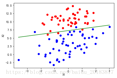
showLogRegres(optimalWeights, train_x, train_y)

都选择迭代330次，对比三种方法的正确率：

左一图选择迭代次数maxIter: 330 选择的方法为：梯度下降algorilthm

正确率为：The classify accuracy is: 95.000%

右一图选择迭代次数maxIter: 330 选择的方法为：随机梯度下降

正确率为：The classify accuracy is: 97.000%

左二图选择迭代次数maxIter: 330 选择的方法为：平稳随机梯度下降

The classify accuracy is: 95.000%

结论：随机梯度下降的正确率最高达到了97%，更适合此场景下的数据挖掘。

机器学习算法与Python实践之逻辑回归（Logistic Regression）

猜你喜欢