版权声明:本文为博主原创文章,未经博主允许不得转载。 https://blog.csdn.net/luyaran/article/details/82785185
当对真实世界数据建模进行回归分析时,我们观察到模型的方程很少是给出线性图的线性方程。 反而是在大多数情况下,现实世界数据模型的方程式涉及更高程度的数学函数,如3或sin函数的指数。 在这种情况下,模型的曲线给出了曲线而不是线性。线性和非线性回归的目标是调整模型参数的值以找到最接近您的数据的线或曲线。当找到这些值时,我们才能够准确估计响应变量。我们这次呢,就来了解下最小二乘回归。
在最小二乘回归中,我们建立了一个回归模型,不同点与回归曲线的垂直距离的平方和之和最小化。 我们通常从定义的模型开始,并假设系数的一些值, 然后就会应用R中的nls()函数来获得更准确的值以及置信区间,来看下语法:
nls(formula, data, start)参数描述如下:
- formula - 是包含变量和参数的非线性模型公式。
- data - 是用于评估(计算)公式中的变量的数据帧。
- start - 是起始估计的命名列表或命名数字向量。
来看一个数学方程式:
a = b1*x^2+b2根据上述的方程式,我们来看一个假设其系数的初始值的非线性模型。首先我们可以先假设初始系数为1和3,并将这些值拟合成nls()函数,如下:
setwd("D:/r_file")
xvalues <- c(1.6,2.1,2,2.23,3.71,3.25,3.4,3.86,1.19,2.21)
yvalues <- c(5.19,7.43,6.94,8.11,18.75,14.88,16.06,19.12,3.21,7.58)

# Give the chart file a name.
png(file = "nls.png")


# Plot these values.
plot(xvalues,yvalues)


# Take the assumed values and fit into the model.
model <- nls(yvalues ~ b1*xvalues^2+b2,start = list(b1 = 1,b2 = 3))

# Plot the chart with new data by fitting it to a prediction from 100 data points.
new.data <- data.frame(xvalues = seq(min(xvalues),max(xvalues),len = 100))
lines(new.data$xvalues,predict(model,newdata = new.data))

# Save the file.
dev.off()

# Get the sum of the squared residuals.
print(sum(resid(model)^2))

# Get the confidence intervals on the chosen values of the coefficients.
print(confint(model))
输出的结果如下所示:
[1] 1.081935
Waiting for profiling to be done...
       2.5%    97.5%
b1 1.137708 1.253135
b2 1.497364 2.496484
产生的图片如下:
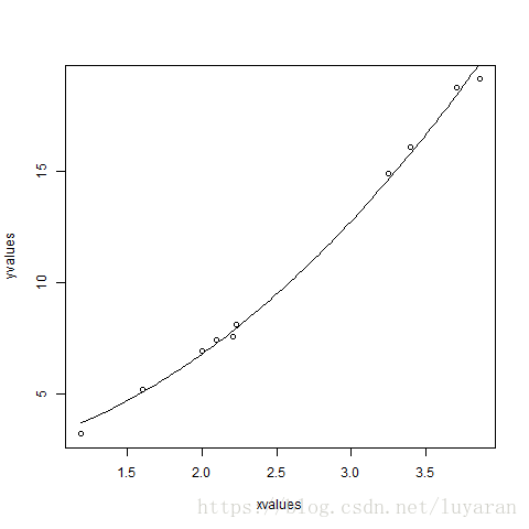
根据上面输出的结果,我们可以得出结论,那就是,b1的值更接近于1,而b2的值更接近于2而不是3。
好啦,本次记录就到这里了。
如果感觉不错的话,请多多点赞支持哦。。。