最小二乘法及线性回归

使用最小二乘法推导出来的关于系数的矩阵公式（\(\theta=(X^TX)^{-1}X^TY\)）也就是我们常说的正规方程。最小二乘法在回归模型中主要是优化拟合函数(此外还可以使用梯度下降法、随机梯度下降法等优化算法来计算函数参数），使得拟合函数能够更好的表达数据。本文将依据正规方程做一简单的线性回归

首先先导入需要用到的包

import numpy as np
import matplotlib.pyplot as plt
from sklearn.datasets import make_regression
from sklearn.model_selection import train_test_split
from sklearn import linear_model

首先请上我们的主角--正规方程，依据上面的公式，我们可以有如下表达：

class OLSRegression:
    def __init__(self,fit_intercept = True):
        self.beta = None
        self.fit_intercept = fit_intercept
    def fit(self,X,y):
        if self.fit_intercept:
            X = np.c_[np.ones(X.shape[0]),X]
        pseudo_inverse = np.dot(np.linalg.inv(np.dot(X.T,X)),X.T)
        self.beta = np.dot(pseudo_inverse,y)
    def predict(self,X):
        if self.fit_intercept:
            X=np.c_[np.ones(X.shape[0]),X]
        return np.dot(X,self.beta)

现在来造数据，将采用sklearn.datasets中的make_regression()方法生成线性回归所需要的数据，并使用sklearn.model_selection中的train_test_split将数据集按7:3的比例分为训练集和测试集。

def random_regression_problem(n_samples,n_features,n_targets,intercept=0,std = 1,seed=0):
    X,y,coef = make_regression(
        n_samples=n_samples,
        n_features = n_features,
        n_targets=n_targets,
        bias=intercept,
        noise=std,
        coef=True,
        random_state=seed,
    )
    X_train,X_test,y_train,y_test=train_test_split(X,y,test_size = 0.3,random_state=seed)
    return X_train,y_train,X_test,y_test

有了数据，我们就要使用正规矩阵来求的拟合函数的参数并利用这些参数进行预测，当然我们都希望最后显示的结果能够更加直观，这里利用matplotlib.pyplot对生成数据以及预测数据进行可视化显示，此外，既然上面用到了sklearn，当然想比较下sklearn中的LinearRegression预测的结果是否和我们的一样了。

def plot_regression():
    np.random.seed(1234)
    fig,axes = plt.subplots(2,2)
    
    for i ,ax in enumerate(axes.flatten()):
        n_samples = 50
        n_features=1
        n_targets=1
        intercept=np.random.rand() * np.random.randint(-300,300)
        std = np.random.randint(0,100)
        X_train,y_train,X_test,y_test = random_regression_problem(n_samples,n_features,n_targets,intercept=intercept,std = std,seed=i)
        olsr = OLSRegression(fit_intercept=True)
        olsr.fit(X_train,y_train)
        y_pred = olsr.predict(X_test)
        loss = np.mean((y_test - y_pred)**2)
        xmin = min(X_test) - 0.1 *(max(X_test) - min(X_test))
        xmax = max(X_test) - 0.1 *(max(X_test) - min(X_test))
        X_plot= np.linspace(xmin,xmax,1000)
        y_plot = olsr.predict(X_plot)
        ax.scatter(X_test,y_test,alpha = 0.5)
        ax.scatter(X_plot,y_plot,label = "My linear",alpha = 0.5)
       
        clf = linear_model.LinearRegression()
        clf.fit(X_train,y_train)
        y_pred_sklearn = clf.predict(X_test)
        loss_sklearn = np.mean((y_pred_sklearn - y_test)**2)
        y_pred_sklearn_plot = clf.predict(X_plot)
        ax.scatter(X_plot,y_pred_sklearn_plot,label = "sklearn linear",alpha = 0.5)
       
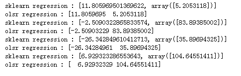
        print("sklearn regression :",[clf.intercept_,clf.coef_])
        print("olsr regression :",olsr.beta)
        
        ax.legend()
        ax.set_title("MSE\n OLSR:{:.2f} Sklearn:{:.2f}".format(loss,loss_sklearn))
        ax.xaxis.set_ticklabels([])
        ax.yaxis.set_ticklabels([])
    plt.tight_layout()#目的让显示的图不那么紧凑

来进行调用：

plot_regression()

先来看下这两种方法得到参数表达：

可视化显示：

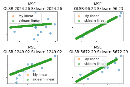
由两种方法求得的参数可以得出，这种方法是一样的，因此，在可视化显示中由于预测值相同，则一种方法得到的预测值会覆盖掉另一种预测值，且均值误差（MSE）同样相同

最小二乘法及线性回归

猜你喜欢