基于Scikit-learn实现回归模型——房价预测

一、收集房屋数据集

二、导入房屋数据集

import pandas as pd
df = pd.read_csv('house_data.csv')

三、可视化房屋数据集特征

import matplotlib.pyplot as plt
import seaborn as sns
sns.set(context = 'notebook')
cols = ['MEDV','LSTAT', 'AGE', 'DIS', 'CRIM', 'TAX', 'RM']
sns.pairplot(df[cols], size=2.5)

显示如下图所示的相互关系图

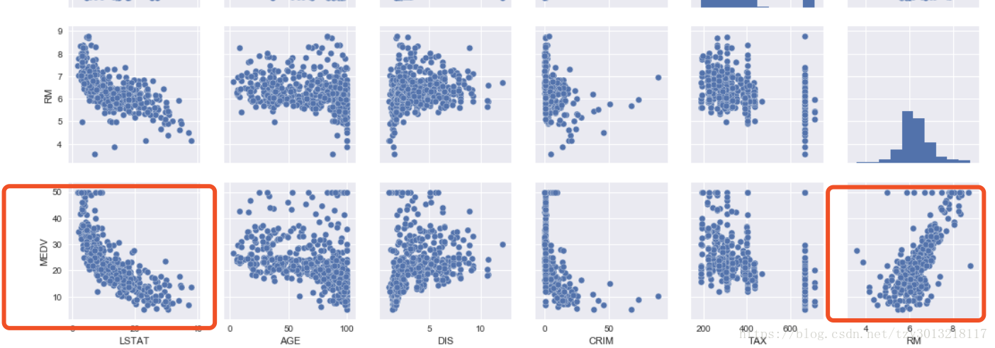
其中MEDV为房屋平均房价，LSTAT为房屋所在地区的人口比例，RM为房间数。不难发现 MEDV 与LSTAT存在反相关关系，MEDV 与RM存在正相关关系。

四、使用sklearn 构建回归模型

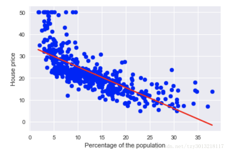
1.构建房价（MEDV）与人口比例 (LSTAT) 的线性模型

from sklearn.linear_model import LinearRegression
sk_model = LinearRegression()
X = df[['LSTAT']].values
y = df['MEDV'].values
sk_model.fit(X, y)
print('Slope: %.3f' % sk_model.coef_[0]) #斜率
print('Intercept : %.3f' % sk_model.intercept_) #截距

输出斜率

Slope: -0.950

输出截距

Intercept : 34.554

然后，定义画出回归函数模型的函数

def Regression_plot(X, y, model):
    plt.scatter(X, y, c='blue')
    plt.plot(X, model.predict(X), color='red')
    return None

调用此函数

Regression_plot(X, y, sk_model)
plt.xlabel('Percentage of the population')
plt.ylabel('House price')

输出结果如下

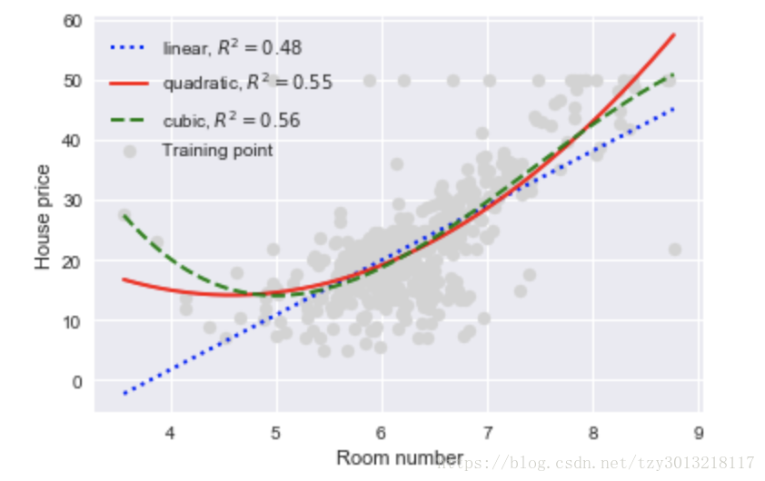
2.构建房价（MEDV）与房间数量 (RM) 的非线性模型

X = df[['RM']].values
y = df['MEDV'].values
Regression_model = LinearRegression() #线性模型
from sklearn.preprocessing import PolynomialFeatures 
quadratic = PolynomialFeatures(degree=2) #二次多项式模型
cubic = PolynomialFeatures(degree=3) #三次多项式模型
X_squared = quadratic.fit_transform(X)
X_cubic = cubic.fit_transform(X)
#相应的X变量进行二次和三次的数据预处理
X_fit = np.arange(X.min(), X.max(), 0.01)[:, np.newaxis]
Linear_model = Regression_model.fit(X, y)
y_line_fit = Linear_model.predict(X_fit)
linear_r2 = r2_score(y, Linear_model.predict(X))
Squared_model = Regression_model.fit(X_squared, y)
y_quad_fit = Squared_model.predict(quadratic.fit_transform(X_fit))
quadratic_r2 = r2_score(y, Squared_model.predict(X_squared))
Cubic_model = Regression_model.fit(X_cubic, y)
y_cubic_fit = Cubic_model.predict(cubic.fit_transform(X_fit))
cubic_r2 = r2_score(y, Cubic_model.predict(X_cubic))

然后，画出拟合结果

plt.scatter(X, y, label='Training point', color='lightgray')
plt.plot(X_fit, y_line_fit, label='linear, $R^2=%.2f$' % linear_r2, color='blue', 
         lw=2, linestyle=':')
plt.plot(X_fit, y_quad_fit, label='quadratic, $R^2=%.2f$' % quadratic_r2, color='red', 
         lw=2, linestyle='-')
plt.plot(X_fit, y_cubic_fit, label='cubic, $R^2=%.2f$' % cubic_r2, color='green', 
         lw=2, linestyle='--')
plt.xlabel('Room number')
plt.ylabel('House price')
plt.legend(loc = 'upper left')

结果如下图所示

五、自己实现线性模型需要的额外操作

如果自己实现线性回归函数，要对数据进行，数据归一化（使特征数据方差为1，均值为0）

一般使用fit_transform()函数和transform()函数进行数据归一化操作，其中：

1）fit_transform()的作用就是先拟合数据，然后转化它将其转化为标准形式

2）tranform()的作用是通过找中心和缩放等实现标准化

为了数据归一化（使特征数据方差为1，均值为0），我们需要计算特征数据的均值μ和方差σ^2，再使用下面的公式进行归一化：

六、交叉验证

待更新。。。。。。

基于Scikit-learn实现回归模型——房价预测

猜你喜欢