2. Gradient descent in practice
2.1 Feature Scaling
让特征们的取值处于同一个范围里面,可以加快梯度下降法的收敛速度。

降低了收敛的速度。 如果将这两个特征scale到同一个范围里面,那么这个椭圆将变成正圆,从边缘向着中心的路程就是半径的距离,变得相当“平坦顺利”,如上图所示。

关于Learning Rate的选择


注意分母使用范围差(最大值-最小值)或者是标准差的结果是不一样的,根据需要选择。
Thank you to Machine Learning Mentor, Tom Mosher, for compiling this list
Subject: Confused about "h(x) = theta' * x" vs. "h(x) = X * theta?"
Text:
The lectures and exercise PDF files are based on Prof. Ng's feeling that novice programmers will adapt to for-loop techniques more readily than vectorized methods. So the videos (and PDF files) are organized toward processing one training example at a time. The course uses column vectors (in most cases), so h (a scalar for one training example) is theta' * x.
Lower-case x typically indicates a single training example.
The more efficient vectorized techniques always use X as a matrix of all training examples, with each example as a row, and the features as columns. That makes X have dimensions of (m x n). where m is the number of training examples. This leaves us with h (a vector of all the hypothesis values for the entire training set) as X * theta, with dimensions of (m x 1).
X (as a matrix of all training examples) is denoted as upper-case X.
Throughout this course, dimensional analysis is your friend.

平均值为 (7921+5184+8836+4761)/4=6675.5
Max-Min=8836-4761=4075
(4761-6675.5)/4075=-0.46957
保留两位小数为-0.47

x= m*(n+1) 14x4
y = X * thetaT, 14x4 4x1 = 14x1
theta 1*(n+1) 1x4
网友上课笔记:
Programming Assignment
1. 加载并显示数据
clear ; close all; clc
data = load('ex1data1.txt');
% 获取两列
X = data(:, 1); y = data(:, 2);
plotData(X, y);


function plotData(x, y)

figure;

plot(x, y, 'rx', 'MarkerSize', 10);
ylabel('Profit in $10,000s');
xlabel('Population of City in 10,000s');

end
这里h(x)在上图中是表示的为theta的转置乘以x,而程序中则是X * theta,原因在上面的的助教问答中已经提到了,前者是表示单个,而后面的是矩阵。
function J = computeCost(X, y, theta)

m = length(y); % number of training examples

J = 0;

predictions = X * theta;
sqrErrors = (predictions - y) .^ 2;
J = 1 / (2 * m) * sum(sqrErrors)

end%% =================== Part 3: Cost and Gradient descent ===================
X = [ones(m, 1), data(:,1)]; % Add a column of ones to x
theta = zeros(2, 1); % initialize fitting parameters, 数据只有两行
% Some gradient descent settings
iterations = 1500;
alpha = 0.01;
fprintf('\nTesting the cost function ...\n')
% compute and display initial cost
J = computeCost(X, y, theta);
fprintf('With theta = [0 ; 0]\nCost computed = %f\n', J);
fprintf('Expected cost value (approx) 32.07\n');
% further testing of the cost function
J = computeCost(X, y, [-1 ; 2]);
fprintf('\nWith theta = [-1 ; 2]\nCost computed = %f\n', J);
fprintf('Expected cost value (approx) 54.24\n');function [theta, J_history] = gradientDescent(X, y, theta, alpha, num_iters)
m = length(y); % number of training examples
J_history = zeros(num_iters, 1);
for iter = 1:num_iters
S = (1 / m) * (X' * (X * theta - y));
theta = theta - alpha .* S;
J_history(iter) = computeCost(X, y, theta);
end
end
% run gradient descent
theta = gradientDescent(X, y, theta, alpha, iterations);
% print theta to screen
fprintf('Theta found by gradient descent:\n');
fprintf('%f\n', theta);
fprintf('Expected theta values (approx)\n');
fprintf(' -3.6303\n 1.1664\n\n');
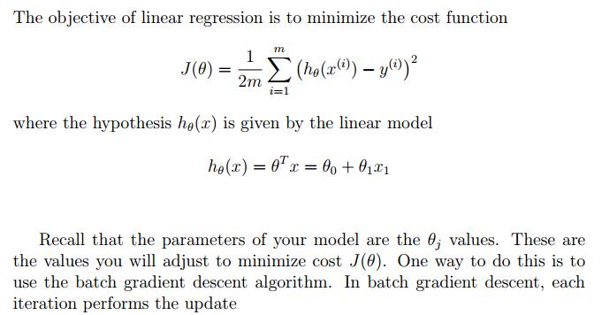
% Plot the linear fit
hold on; % keep previous plot visible
plot(X(:,2), X*theta, '-')
legend('Training data', 'Linear regression')
hold off % don't overlay any more plots on this figure
% Predict values for population sizes of 35,000 and 70,000
predict1 = [1, 3.5] *theta;
fprintf('For population = 35,000, we predict a profit of %f\n',...
predict1*10000);
predict2 = [1, 7] * theta;
fprintf('For population = 70,000, we predict a profit of %f\n',...
predict2*10000);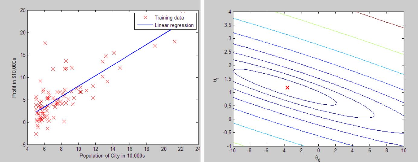
多变量的线性回归

使用不同的Learning Rate可以看到不同的J,利用方程求导和梯度下降对同一例子进行预测,结果如2,4箭头,较为相近。但是发现他们的theta(1,3)不一样。不同方法得到的模型不一样,但是结果类似,殊途同归。