欢迎来到第三周的课程,在这一周的任务里,你将建立一个只有一个隐含层的神经网络。相比于之前你实现的逻辑回归有很大的不同。
你将会学习一下内容:
- 用一个隐含层的神经网络实现一个二分类。
- 利用非线性的激活函数单元。
- 计算交叉熵损失函数。
- 实现向前传播和向后传播。
1 函数包
# Package imports
import numpy as np
import matplotlib.pyplot as plt
from testCases import *
import sklearn
import sklearn.datasets
import sklearn.linear_model
from planar_utils import plot_decision_boundary, sigmoid, load_planar_dataset, load_extra_datasets

%matplotlib inline

np.random.seed(1) # set a seed so that the results are consistent
2 数据
X, Y = load_planar_dataset()

# Visualize the data:
plt.scatter(X[0, :], X[1, :], c=Y, s=40, cmap=plt.cm.Spectral);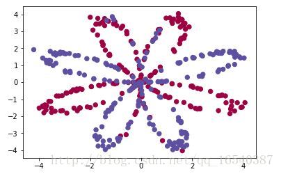
能将得到
1. 一个包含(x1,x2)的特征矩阵。
2. 一个包含(0,1)的特征向量。
练习:你有多少训练集,他们的大小是多少?
### START CODE HERE ### (≈ 3 lines of code)
shape_X = X.shape
shape_Y = Y.shape

m = shape_X[1]  # training set size
### END CODE HERE ###

print ('The shape of X is: ' + str(shape_X))
print ('The shape of Y is: ' + str(shape_Y))
print ('I have m = %d training examples!' % (m))
输出:
The shape of X is: (2L, 400L)
The shape of Y is: (1L, 400L)
I have m = 400 training examples!
3 简单的逻辑回归
在进行今天的作业之前,先看一下,逻辑回归在这个问题上的表现。
# Train the logistic regression classifier
clf = sklearn.linear_model.LogisticRegressionCV();
clf.fit(X.T, Y.T);

# Plot the decision boundary for logistic regression
plot_decision_boundary(lambda x: clf.predict(x), X, Y)
plt.title("Logistic Regression")

# Print accuracy
LR_predictions = clf.predict(X.T)
print ('Accuracy of logistic regression: %d ' % float((np.dot(Y,LR_predictions) + np.dot(1-Y,1-LR_predictions))/float(Y.size)*100) +
'% ' + "(percentage of correctly labelled datapoints)")输出:

说明:因为数据集是非线性可分的,所以,在这个数据集上表现较差。
4 神经网络模型
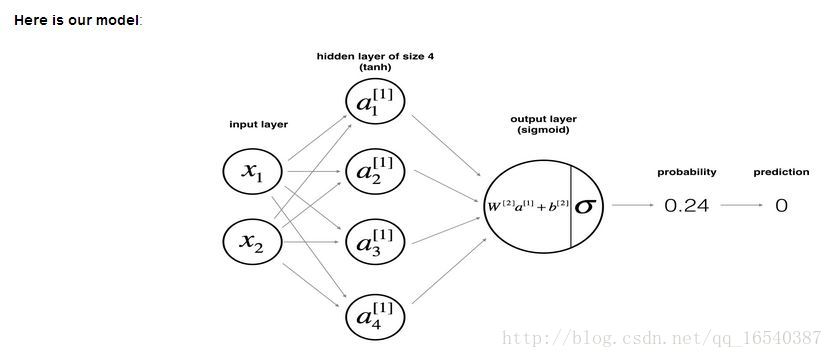
回忆:通常神经网络建立的方法。
- 定义神经网络的结构(输入层,输出层,隐含层个数)。
- 初始化模型参数。
- 循环:
—实现向前传播。
—计算损失函数。
—为了得到梯度值,实现向后传播。
—更新参数(梯度下降)
4.1 定义神经网络结构
练习:定义三个结构变量
# GRADED FUNCTION: layer_sizes

def layer_sizes(X, Y):
    """
    Arguments:
    X -- input dataset of shape (input size, number of examples)
    Y -- labels of shape (output size, number of examples)

    Returns:
    n_x -- the size of the input layer
    n_h -- the size of the hidden layer
    n_y -- the size of the output layer
    """
    ### START CODE HERE ### (≈ 3 lines of code)
    n_x = X.shape[0] # size of input layer
    n_h = 4
    n_y = Y.shape[0] # size of output layer
    ### END CODE HERE ###
    return (n_x, n_h, n_y)
4.2 初始化模型参数
练习:实现initialize_parameters()函数功能
说明:
- 用 np.random.randn(a,b) * 0.01随机的初始化权重矩阵
- 用np.zeros((a,b))初始化偏置向量
# GRADED FUNCTION: initialize_parameters

def initialize_parameters(n_x, n_h, n_y):
    """
    Argument:
    n_x -- size of the input layer
    n_h -- size of the hidden layer
    n_y -- size of the output layer

    Returns:
    params -- python dictionary containing your parameters:
                    W1 -- weight matrix of shape (n_h, n_x)
                    b1 -- bias vector of shape (n_h, 1)
                    W2 -- weight matrix of shape (n_y, n_h)
                    b2 -- bias vector of shape (n_y, 1)
    """

    np.random.seed(2) # we set up a seed so that your output matches ours although the initialization is random.

    ### START CODE HERE ### (≈ 4 lines of code)
    W1 = np.random.randn(n_h,n_x) * 0.01
    b1 = np.zeros((n_h,1))
    W2 = np.random.randn(n_y,n_h) * 0.01
    b2 = np.zeros((n_y,1))
    ### END CODE HERE ###

    assert (W1.shape == (n_h, n_x))
    assert (b1.shape == (n_h, 1))
    assert (W2.shape == (n_y, n_h))
    assert (b2.shape == (n_y, 1))

    parameters = {"W1": W1,
                  "b1": b1,
                  "W2": W2,
                  "b2": b2}

    return parameters
输出:
W1 = [[-0.00416758 -0.00056267]
[-0.02136196 0.01640271]
[-0.01793436 -0.00841747]
[ 0.00502881 -0.01245288]]
b1 = [[ 0.]
[ 0.]
[ 0.]
[ 0.]]
W2 = [[-0.01057952 -0.00909008 0.00551454 0.02292208]]
b2 = [[ 0.]]
4.3循环
问题:实现 forward_propagation().
- 从字典“parameters”中检索每个参数。
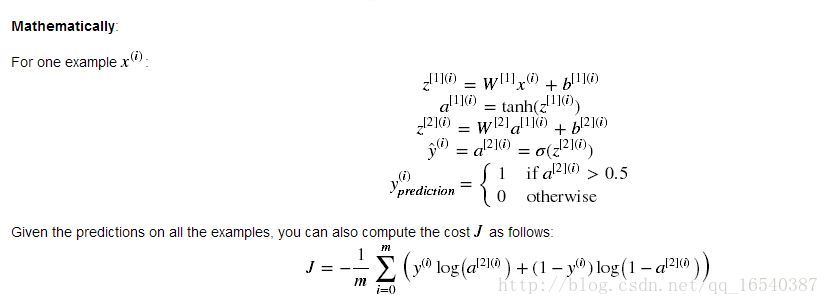
- 实现向前传播。计算Z1,A1,Z2,A2(这是所有你对训练集的所有例子的预测的向量)。
- 反向传播所需的值存储在“cache”中。cache将作为反向传播函数的一个输入。
# GRADED FUNCTION: forward_propagation

def forward_propagation(X, parameters):
    """
    Argument:
    X -- input data of size (n_x, m)
    parameters -- python dictionary containing your parameters (output of initialization function)

    Returns:
    A2 -- The sigmoid output of the second activation
    cache -- a dictionary containing "Z1", "A1", "Z2" and "A2"
    """
    # Retrieve each parameter from the dictionary "parameters"
    ### START CODE HERE ### (≈ 4 lines of code)
    W1 = parameters["W1"]
    b1 = parameters["b1"]
    W2 = parameters["W2"]
    b2 = parameters["b2"]
    ### END CODE HERE ###

    # Implement Forward Propagation to calculate A2 (probabilities)
    ### START CODE HERE ### (≈ 4 lines of code)
    Z1 = np.dot(W1,X) + b1
    A1 = np.tanh(Z1)
    Z2 = np.dot(W2,A1) + b2
    A2 = sigmoid(Z2)
    ### END CODE HERE ###

    assert(A2.shape == (1, X.shape[1]))

    cache = {"Z1": Z1,
             "A1": A1,
             "Z2": Z2,
             "A2": A2}

return A2, cache输出:
(-0.00049975577774199022, -0.00049696335323177901, 0.00043818745095914653, 0.50010954685243103)
计算出A2后,你将计算损失函数
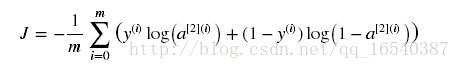
练习:实现 compute_cost(),计算损失函数
# GRADED FUNCTION: compute_cost

def compute_cost(A2, Y, parameters):
    """
    Computes the cross-entropy cost given in equation (13)

    Arguments:
    A2 -- The sigmoid output of the second activation, of shape (1, number of examples)
    Y -- "true" labels vector of shape (1, number of examples)
    parameters -- python dictionary containing your parameters W1, b1, W2 and b2

    Returns:
    cost -- cross-entropy cost given equation (13)
    """

    m = Y.shape[1] # number of example

    # Compute the cross-entropy cost
     ### START CODE HERE ### (≈ 2 lines of code)
    logprobs = np.multiply(np.log(A2),Y) + np.multiply(np.log(1 - A2),1 - Y)
    cost = - np.sum(logprobs) / m
    ### END CODE HERE ###

    cost = np.squeeze(cost)     # makes sure cost is the dimension we expect.
                                # E.g., turns [[17]] into 17
    assert(isinstance(cost, float))

    return cost
输出:cost = 0.692919893776
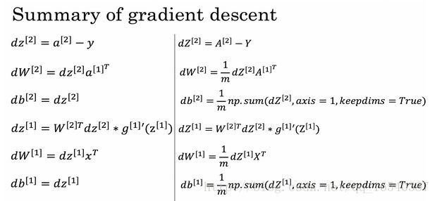
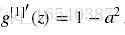
问题:实现反向传播函数 backward_propagation()
其中, tanh激活函数的导数为
# GRADED FUNCTION: backward_propagation

def backward_propagation(parameters, cache, X, Y):
    """
    Implement the backward propagation using the instructions above.

    Arguments:
    parameters -- python dictionary containing our parameters
    cache -- a dictionary containing "Z1", "A1", "Z2" and "A2".
    X -- input data of shape (2, number of examples)
    Y -- "true" labels vector of shape (1, number of examples)

    Returns:
    grads -- python dictionary containing your gradients with respect to different parameters
    """
    m = X.shape[1]

    # First, retrieve W1 and W2 from the dictionary "parameters".
    ### START CODE HERE ### (≈ 2 lines of code)
    W1 = parameters["W1"]
    W2 = parameters["W2"]
    ### END CODE HERE ###

    # Retrieve also A1 and A2 from dictionary "cache".
    ### START CODE HERE ### (≈ 2 lines of code)
    A1 = cache["A1"]
    A2 = cache["A2"]
    ### END CODE HERE ###

    # Backward propagation: calculate dW1, db1, dW2, db2.
    ### START CODE HERE ### (≈ 6 lines of code, corresponding to 6 equations on slide above)
    dZ2 = A2 - Y
    dW2 =  np.dot(dZ2,A1.T)/m
    db2 = np.sum(dZ2,axis=1,keepdims=True)/m
    dZ1 = np.multiply(np.dot(W2.T,dZ2), (1 - np.power(A1, 2)))
    dW1 = np.dot(dZ1,X.T)/m
    db1 =  np.sum(dZ1,axis=1,keepdims=True)/m
    ### END CODE HERE ###

    grads = {"dW1": dW1,
             "db1": db1,
             "dW2": dW2,
             "db2": db2}

    return grads
输出:
dW1 = [[ 0.01018708 -0.00708701]
[ 0.00873447 -0.0060768 ]
[-0.00530847 0.00369379]
[-0.02206365 0.01535126]]
db1 = [[-0.00069728]
[-0.00060606]
[ 0.000364 ]
[ 0.00151207]]
dW2 = [[ 0.00363613 0.03153604 0.01162914 -0.01318316]]
db2 = [[ 0.06589489]]
问题:利用地图下降,实现更新法则。你可以利用 (dW1, db1, dW2, db2) 去更新 (W1, b1, W2, b2).
通常的梯度下降准则:
说明:梯度下降和学习速率关系很大。
# GRADED FUNCTION: update_parameters

def update_parameters(parameters, grads, learning_rate = 1.2):
    """
    Updates parameters using the gradient descent update rule given above

    Arguments:
    parameters -- python dictionary containing your parameters
    grads -- python dictionary containing your gradients

    Returns:
    parameters -- python dictionary containing your updated parameters
    """
    # Retrieve each parameter from the dictionary "parameters"
    ### START CODE HERE ### (≈ 4 lines of code)
    W1 = parameters["W1"]
    b1 = parameters["b1"]
    W2 = parameters["W2"]
    b2 = parameters["b2"]
    ### END CODE HERE ###

    # Retrieve each gradient from the dictionary "grads"
    ### START CODE HERE ### (≈ 4 lines of code)
    dW1 = grads["dW1"]
    db1 = grads["db1"]
    dW2 = grads["dW2"]
    db2 = grads["db2"]
    ## END CODE HERE ###

    # Update rule for each parameter
    ### START CODE HERE ### (≈ 4 lines of code)
    W1 = W1 - learning_rate * dW1
    b1 = b1 - learning_rate * db1
    W2 = W2 - learning_rate * dW2
    b2 = b2 - learning_rate * db2
    ### END CODE HERE ###

    parameters = {"W1": W1,
                  "b1": b1,
                  "W2": W2,
                  "b2": b2}

return parameters输出:
W1 = [[-0.00643025 0.01936718]
[-0.02410458 0.03978052]
[-0.01653973 -0.02096177]
[ 0.01046864 -0.05990141]]
b1 = [[ -1.02420756e-06]
[ 1.27373948e-05]
[ 8.32996807e-07]
[ -3.20136836e-06]]
W2 = [[-0.01041081 -0.04463285 0.01758031 0.04747113]]
b2 = [[ 0.00010457]]
4.4 综合前面三部分 nn_model()
问题:建立神经学习网络
# GRADED FUNCTION: nn_model

def nn_model(X, Y, n_h, num_iterations = 10000, print_cost=False):
    """
    Arguments:
    X -- dataset of shape (2, number of examples)
    Y -- labels of shape (1, number of examples)
    n_h -- size of the hidden layer
    num_iterations -- Number of iterations in gradient descent loop
    print_cost -- if True, print the cost every 1000 iterations

    Returns:
    parameters -- parameters learnt by the model. They can then be used to predict.
    """

    np.random.seed(3)
    n_x = layer_sizes(X, Y)[0]
    n_y = layer_sizes(X, Y)[2]

    # Initialize parameters, then retrieve W1, b1, W2, b2. Inputs: "n_x, n_h, n_y". Outputs = "W1, b1, W2, b2, parameters".
    ### START CODE HERE ### (≈ 5 lines of code)
    parameters = initialize_parameters(n_x, n_h, n_y)
    W1 = parameters["W1"]
    b1 = parameters["b1"]
    W2 = parameters["W2"]
    b2 = parameters["b2"]
    ### END CODE HERE ###

    # Loop (gradient descent)

    for i in range(0, num_iterations):

        ### START CODE HERE ### (≈ 4 lines of code)
        # Forward propagation. Inputs: "X, parameters". Outputs: "A2, cache".
        A2, cache = forward_propagation(X, parameters)

        # Cost function. Inputs: "A2, Y, parameters". Outputs: "cost".
        cost = compute_cost(A2, Y, parameters)

        # Backpropagation. Inputs: "parameters, cache, X, Y". Outputs: "grads".
        grads = backward_propagation(parameters, cache, X, Y)

        # Gradient descent parameter update. Inputs: "parameters, grads". Outputs: "parameters".
        parameters = update_parameters(parameters, grads ,)

        ### END CODE HERE ###

        # Print the cost every 1000 iterations
        if print_cost and i % 1000 == 0:
            print ("Cost after iteration %i: %f" %(i, cost))

    return parameters
输出:
W1 = [[-4.18494502 5.33220306]
[-7.52989352 1.24306198]
[-4.19295477 5.32631754]
[ 7.52983748 -1.24309404]]
b1 = [[ 2.32926814]
[ 3.79459053]
[ 2.3300254 ]
[-3.79468789]]
W2 = [[-6033.83672183 -6008.12981297 -6033.10095335 6008.0663689 ]]
b2 = [[-52.666077]]
4.5 预测
问题:通过建立函数 predict()进行预测。利用向前传播进行预测。
# GRADED FUNCTION: predict

def predict(parameters, X):
    """
    Using the learned parameters, predicts a class for each example in X

    Arguments:
    parameters -- python dictionary containing your parameters
    X -- input data of size (n_x, m)

    Returns

    predictions -- vector of predictions of our model (red: 0 / blue: 1)
    """

    # Computes probabilities using forward propagation, and classifies to 0/1 using 0.5 as the threshold.
  ### START CODE HERE ### (≈ 2 lines of code)
    A2, cache = forward_propagation(X, parameters)
    predictions = np.round(A2)
    ### END CODE HERE ###

    return predictions
输出:predictions mean = 0.666666666667
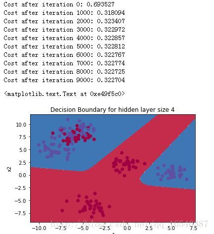
4.6预测原数据
# Build a model with a n_h-dimensional hidden layer
parameters = nn_model(X, Y, n_h = 4, num_iterations = 10000, print_cost=True)

# Plot the decision boundary
plot_decision_boundary(lambda x: predict(parameters, x.T), X, Y)
plt.title("Decision Boundary for hidden layer size " + str(4))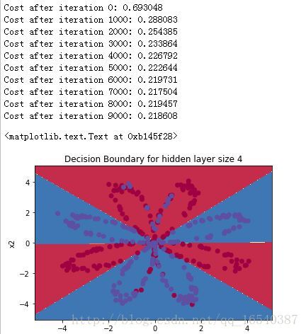
# Print accuracy
predictions = predict(parameters, X)
print ('Accuracy: %d' % float((np.dot(Y,predictions.T) + np.dot(1-Y,1-predictions.T))/float(Y.size)*100) + '%')
输出:Accuracy: 90%
4.7 改变隐含层的大小
# This may take about 2 minutes to run

plt.figure(figsize=(16, 32))
hidden_layer_sizes = [1, 2, 3, 4, 5, 10, 20]
for i, n_h in enumerate(hidden_layer_sizes):
    plt.subplot(5, 2, i+1)
    plt.title('Hidden Layer of size %d' % n_h)
    parameters = nn_model(X, Y, n_h, num_iterations = 5000)
    plot_decision_boundary(lambda x: predict(parameters, x.T), X, Y)
    predictions = predict(parameters, X)
    accuracy = float((np.dot(Y,predictions.T) + np.dot(1-Y,1-predictions.T))/float(Y.size)*100)
    print ("Accuracy for {} hidden units: {} %".format(n_h, accuracy))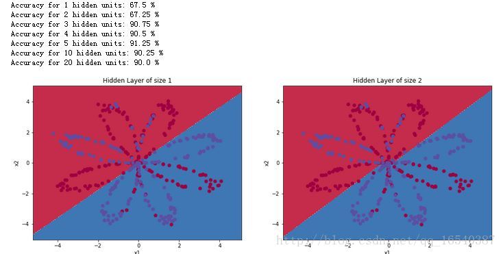
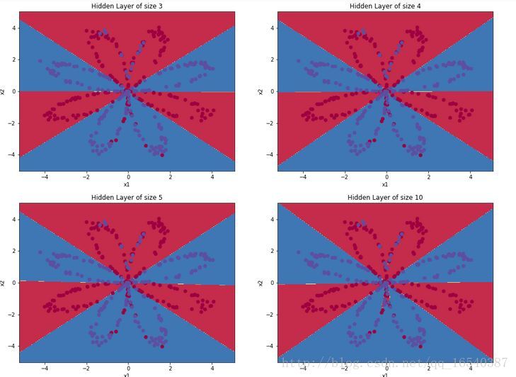
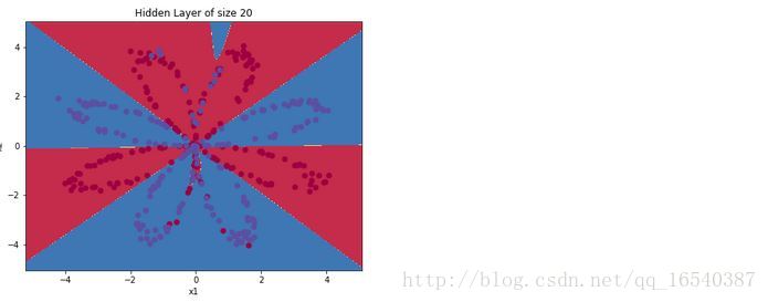
说明:
- 较大的模型(包含更多的隐藏单元)能够更好地适应训练集,直到最终最大的模型超过了数据。
- 最好的隐藏层大小似乎是在nh=5附近。实际上,这里的价值似乎与数据吻合得很好,而不需要引起注意的过度拟合。
- 稍后您还将学习规范化,这使您可以使用非常大的模型(例如nh=50),而不需要太多的过度使用。
5 在其他数据集上的表现
# Datasets
noisy_circles, noisy_moons, blobs, gaussian_quantiles, no_structure = load_extra_datasets()
datasets = {"noisy_circles": noisy_circles,
"noisy_moons": noisy_moons,
"blobs": blobs,
"gaussian_quantiles": gaussian_quantiles}
### START CODE HERE ### (choose your dataset)
dataset = "blobs"
### END CODE HERE ###
X, Y = datasets[dataset]
X, Y = X.T, Y.reshape(1, Y.shape[0])
# make blobs binary
if dataset == "blobs":
Y = Y%2
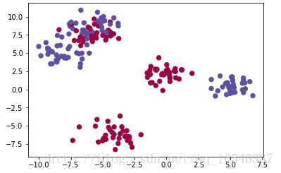
# Visualize the data
plt.scatter(X[0, :], X[1, :], c=Y, s=40, cmap=plt.cm.Spectral);
# Build a model with a n_h-dimensional hidden layer
parameters = nn_model(X, Y, n_h = 4, num_iterations = 10000, print_cost=True)
# Plot the decision boundary
plot_decision_boundary(lambda x: predict(parameters, x.T), X, Y)
plt.title("Decision Boundary for hidden layer size " + str(4))