神经网络与深度学习_神经网络基础_第二周笔记

Supervised learning

Application:

• Standard NN
  • real estate
  • Online advertising
• CNN
  • Photo tagging
• RNN
  • Speech recognition
  • Machine translation
• Custom/hybrid RNNs
  • Autonomous driving

---

Notation

$(x,y), x∈R^{n_x} ,y∈\{0,1\}$
m training example { $(x^{(1)},y^{(1)}),(x^{(2)},y^{(2)}),...,(x^{(m)},y^{(m)})$}
$X= \left[ \begin{matrix} . & . & . & . & .& -\\ . & . & . & . & . &|\\ x^{(1)} & x^{(2)} & ... & ... & x^{(m)} & n_x\\ . & . & . & . & .& | \\ . & . & . & . & .& -\\ <- & & m & & ->& \\ \end{matrix} \right]$
$X∈R^{n_x * m }, Y=[y^{(1)},y^{(2)},..,y^{(m)}], Y∈R^{1* m}$

x.shape(nx,m) y.shape=(1,m)

---

Logistic Regression

$x∈R^{n_x}, want: \hat{y}=P(y=1|x),so 0≤\hat{y}≤1$
$parameters: w∈R^{n_x},b∈R$
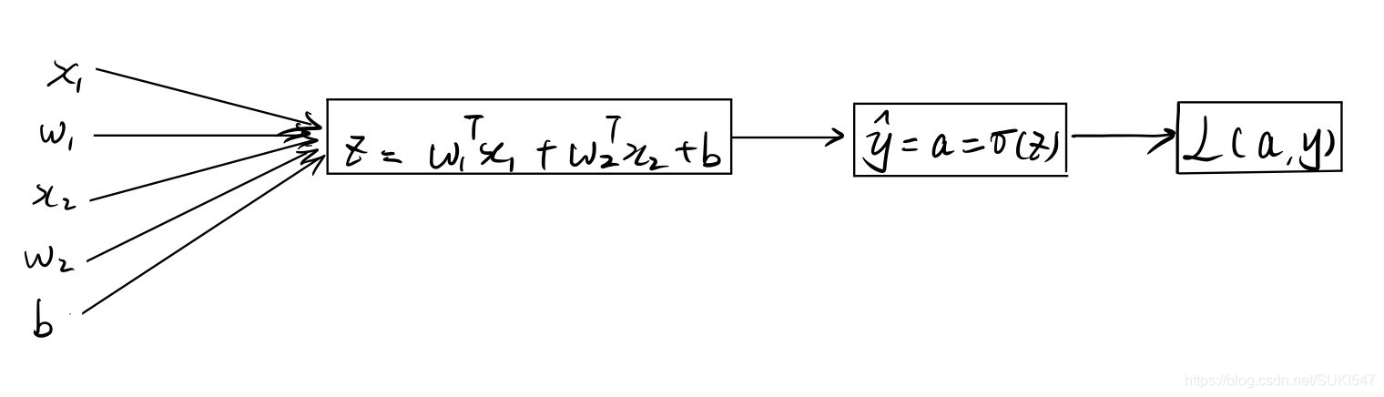
$Output: \hat{y}=\sigma (w^Tx+b)$
$\sigma$ is activation function $\sigma (z)= \frac{1}{1+e^{(-z)}}$

---

Logistic Regression Cost Function

$\hat{y}^{(i)}= \sigma(w^Tx^{(i)}+b)$

given { $(x^{(1)},y^{(1)}),(x^{(2)},y^{(2)}),...,(x^{(m)},y^{(m)})$} want $\hat{y}^{(i)} \approx y^{(i)}$

Measure single training sample

usually can use

$L(\hat{y},y)=\frac{1}{2}(\hat{y}-y)^2$

to measure the gap but later gradient descent may not work well because it’s non-convex function

$\hat{y}=\sigma (w^Tx+b),where: \sigma(z)=\frac{1}{1+e^{-z}},interpret :\hat{y}=P(y=1|x)$
IF $y=1:P(y|x)=\hat{y}$
IF $y=0:P(y|x)=1-\hat{y}$

combine the function above
$P(y|x)=\hat{y}^y(1-\hat{y})^{1-y}$and the $\log$ function is a strictly monotonically increasing function
$\log P(y|x)=y\log\hat{y}+(1-y)\log(1-\hat{y})$then add negative sign because we want the minimum cost, so

$\begin{aligned} -\log P(y|x)=&-[y\log\hat{y}+(1-y)\log(1-\hat{y})]\\ L(\hat{y},y)=&-[y\log\hat{y}+(1-y)\log(1-\hat{y})] \end{aligned}$

this is the cost function with single example

Cost function in m training set

under IID
$P(labels-in-training-set) =\prod_{i=1}^mP(y^{(i)}|x^{(i)})$ to maximizing the training set chance as same as maximizing the $\log$ fun

$\begin{aligned} \log P(labels-in-training-set) =&\log \prod_{i=1}^mP(y^{(i)}|x^{(i)})\\ =&\sum_{i=1}^m \log P(y^{(i)}|x^{(i)})\\ =&\sum_{i=1}^m-L(\hat{y}^{(i)},y^{(i)})\\ =&\frac{1}{m}\sum_{i=1}^m-L(\hat{y}^{(i)},y^{(i)}) \end{aligned}$

add $\frac{1}{m}$ scaling factor to for better scale
so the overall cost function

$J(w,b)=\frac{1}{m}\sum_{i=1}^m L(\hat{y}^{(i)},y^{(i)})$

remove the nagative for minimize the cost function
$J(w,b)$ is convex func, that is the particular reason to be chosen for cost function

---

Gradient Descent

Repeat:{
$w:= w-\alpha \frac{dJ(w,b)}{dw}$
$b:= b-\alpha \frac{dJ(w,b)}{db}$
}
$\alpha$ is the learning rate

Computation Graph

from right to left

$\frac{dL}{da}=-\frac{y}{a}+\frac{1-y}{1-a}$

$\frac {dL}{dz}=\frac{dL}{da}\cdot \frac{da}{dz}=(-\frac{y}{a}+\frac{1-y}{1-a})(a(1-a))=a-y=dz$

$\frac {dL}{dw_{1}}=\frac{dL}{dz}\cdot \frac{dz}{dw_1}=dz \cdot x_1=dw_1$

$\frac {dL}{dw_{2}}=\frac{dL}{dz}\cdot \frac{dz}{dw_2}=dz \cdot x_2=dw_2$

$\frac {dL}{db}=\frac{dL}{dz}\cdot \frac{dz}{db}=dz=db$

so in single example :

$\omega_1:= \omega_1-\alpha dz\cdot x_1$
$\omega_2:= \omega_2-\alpha dz\cdot x_2$
$b:= b-\alpha dz$

---

Gradient descent in m example

$J(w,b)=\frac{1}{m}\sum_{i=1}^mL(a^{(i)},y^{(i)}), a^{(i)}=\hat{y}^{(i)}=\sigma(z^{(i)})=\sigma(\omega^T x^{(i)}+b)$

$\begin{aligned} \frac{dJ(w_1,b)}{dw_1}=&\frac{1}{m}\sum_{i=1}^m \frac {dL(a^{(i)},y^{(i)})}{dw_1}\\ =&\frac{1}{m}\sum_{i=1}^m dw_1^{(i)} -- using (x_1^{(i)},y^{(i)}) \end{aligned}$

J=0 dw1=0 dw2=0 b=0
for i=1 to m
    z[i]=w_T*x[i]+b
    a[i]=sigma(z[i])
    J[i]+=-[y[i]*log(a[i])+(1-y[i])*log(1-a[i])]
    dz[i]=a[i]-y[i]
    for w in wm
       dw[1] += dz[i]*x1[i]
       dw[2] +=dz[i]*x2[i]
       ...
       db +=dz[i]
     end
 end
 dw1=dw1/m dw2=dw2/m db=db/m J=J/m

There are 2 loops ,less efficiency $\longrightarrow$ Vectorization

---

Vectorization

$Z=\omega ^Tx+b$

• non-vectorization

       z=0
       for i in range(nx):
           z += w[i]*x[i]
       z = z+b

• vectorization

  $\omega = \left[ \begin{matrix} . \\ . \\ \omega^{(i)} \\ . \\ . \\ \end{matrix} \right] X = \left[ \begin{matrix} . \\ . \\ x^{(i)} \\ . \\ . \\ \end{matrix} \right] \omega \in R^{n_x},x \in R^{n_x}$

dw=np.zeros(n_x,1) x.shape(n_x,1)

so in code

J=0  b=0
dw=np.zeros(n_x,1)
for i=1 to m //one loop for x
    z[i]=w_T*x[i]+b
    a[i]=sigma(z[i])
    J[i]+=-[y[i]* log(a[i])+(1-y[i])* log(1-a[i])]
    dz[i]=a[i]-y[i]
    dw += dw[i]* x[i]
    db +=dz[i]
 end
 dw=dw/m db=db/m J=J/m

Vectoring Logistic Regression

$z^{(1)}=\omega ^Tx^{(1)}+b ,a^{(1)}=\sigma(z^{(1)})\\ z^{(2)}=\omega ^Tx^{(2)}+b ,a^{(2)}=\sigma(z^{(2)}) \\...$

$X= \left[ \begin{matrix} . & . & . & . & .\\ . & . & . & . & .\\ x^{(1)} & x^{(2)} & ... & ... & x^{(m)} \\ . & . & . & . & .\\ . & . & . & . & .\\ \end{matrix} \right]$

$\begin{aligned} Z=&[z^{(1)},z^{(2)},z^{(3)},...,z^{(m)}]\\=&\omega ^{T}X+[b,b,...,b]\\=&[\omega ^{T}x^{(1)}+b,\omega ^{T}x^{(2)}+b,...,\omega ^{T}x^{(m)}+b] \end{aligned}$

Z =np.dot(w.T,x)+b . //python Broadcasting as a vector

Vecrotring Logistic Regression Gradient Descent

$dz^{(i)}=a^{(i)}-y^{(i)},\\dz=[dz^{(1)},dz^{(2)},...,dz^{(m)}],\\A=[a^{(1)},a^{(2)},..,a^{(m)}],\\Y=[y^{(1)},y^{(2)},...,y^{(m)}] ,\\dz=A-Y\\ db=\frac {1}{m}\sum^m_{i=1} dz^{(i)}$

db=np.sum(dz)/m

$d\omega=\frac{1}{m} \cdot X \cdot dz^T$
$d\omega=\frac{1}{m} \left[ \begin{matrix} . & . & . & . & .\\ . & . & . & . & .\\ x^{(1)} & x^{(2)} & ... & ... & x^{(m)} \\ . & . & . & . & .\\ . & . & . & . & .\\ \end{matrix} \right] \cdot \left[ \begin{matrix} d^{(1)} \\ d^{(2)} \\ .\\ . \\ d^{(m)} \\ \end{matrix} \right]=\frac{1}{m}[x^{(1)}dz^{(1)}+x^{(2)}dz^{(2)}...+x^{(m)}dz^{(m)}]$

for iter in range(2000):
 z=np.dot(W.T,X)+b
 A=sigmoid(z)
 dz=A-Y
 dw=np.dot(X,dz.T)/m
 db=np.sum(dz)/m
 W=W-alpha * dw
 b=b-alpha * db