目录
1.二分分类

2.logistic 回归

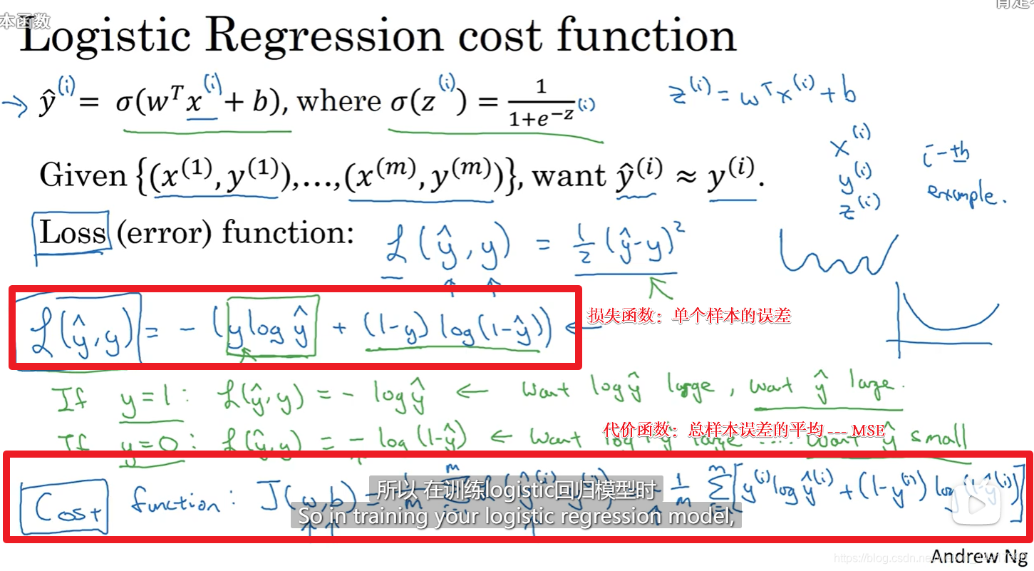
3.logistic 代价函数


4.梯度下降法

5.计算图
可以参考刘普洪老师的计算图

6.logistic回归中的梯度下降法


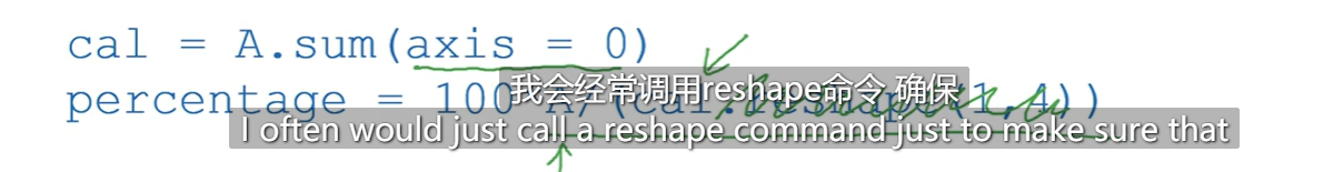
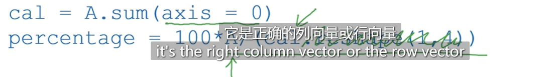
7.向量化


程序第二、六行错误!!!
8.向量化logistic回归


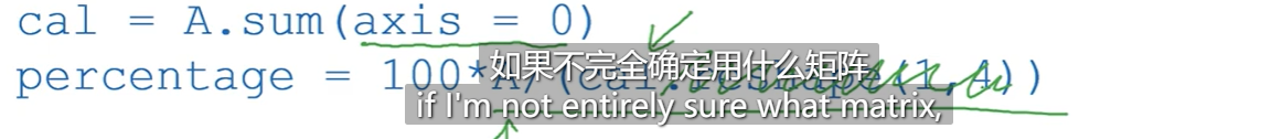
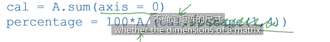
9.Python中的广播


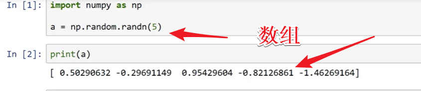
10.python numpy


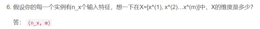
(测验)作业:


(编程)作业
数据集测试:
#! /usr/bin/env python
# -*- coding: utf-8 -*-

"""
============================================
时间:2021.8.15
作者:手可摘星辰不去高声语
文件名:lr_utils.py
功能:引用数据集(训练集 + 测试集),输出数据集的图片和标签
1、Ctrl + Enter      在下方新建行但不移动光标;
2、Shift + Enter     在下方新建行并移到新行行首;
3、Shift + Enter     任意位置换行
4、Ctrl + D          向下复制当前行
5、Ctrl + Y         删除当前行
6、Ctrl + Shift + V  打开剪切板
7、Ctrl + /          注释(取消注释)选择的行;
8、Ctrl + E       可打开最近访问过的文件
9、Double Shift + /  万能搜索
============================================
"""


import numpy as np
import matplotlib.pyplot as plt
import h5py


class Load_data:
    def __init__(self):
        self.train_dataset = h5py.File('datasets/train_catvnoncat.h5', "r")
        self.test_dataset = h5py.File('datasets/test_catvnoncat.h5', "r")

    def load_dataset(self):
        """
        运行文件可以查看函数输出的具体信息
        """
        # your train set features(训练集里面的图像数据:本训练集中209张64×64的图像)
        train_set_x_orig = np.array(self.train_dataset["train_set_x"][:])
        # your train set labels(训练集的图像的分类值:0不是猫,1是猫)
        train_set_y_orig = np.array(self.train_dataset["train_set_y"][:])
        # your test set features(测试集里面的图像数据:本训练集中50张64×64的图像)
        test_set_x_orig = np.array(self.test_dataset["test_set_x"][:])
        # your test set labels(测试集的图像的分类值:0不是猫,1是猫)
        test_set_y_orig = np.array(self.test_dataset["test_set_y"][:])
        # the list of classes(保存的是以bytes类型保存的两个字符串数据,数据为:[b’non-cat’ b’cat’])
        classes = np.array(self.test_dataset["list_classes"][:])

        train_set_y_orig = train_set_y_orig.reshape((1, train_set_y_orig.shape[0]))
        test_set_y_orig = test_set_y_orig.reshape((1, test_set_y_orig.shape[0]))

        return train_set_x_orig, train_set_y_orig, test_set_x_orig, test_set_y_orig, classes


if __name__ == '__main__':
    Load_dataset = Load_data()
    train_set_x_orig, train_set_y_orig, test_set_x_orig, test_set_y_orig, classes = Load_dataset.load_dataset()

    # 查看训练集的信息
    m_train = train_set_y_orig.shape[1]  # 训练集里图片的数量。
    m_test = test_set_y_orig.shape[1]  # 测试集里图片的数量。
    num_px = train_set_x_orig.shape[1]  # 训练、测试集里面的图片的宽度和高度(均为64x64)。

    # 现在看一看我们加载的东西的具体情况
    print("训练集的数量: m_train = " + str(m_train))
    print("测试集的数量 : m_test = " + str(m_test))
    print("每张图片的宽/高 : num_px = " + str(num_px))
    print("每张图片的大小 : (" + str(num_px) + ", " + str(num_px) + ", 3)")
    print("训练集_图片的维数 : " + str(train_set_x_orig.shape))
    print("训练集_标签的维数 : " + str(train_set_y_orig.shape))
    print("测试集_图片的维数: " + str(test_set_x_orig.shape))
    print("测试集_标签的维数: " + str(test_set_y_orig.shape))

    # 查看1:4张图片以及分类
    for numb in range(0, 4):
        plt.subplot(2, 2, numb+1)
        index = numb
        plt.imshow(train_set_x_orig[index])
        # 标题显示训练集的图片的分类
        # np.squeeze表示降维([]-> 数值)
        # decode("utf-8")进行解码(classes是以bytes类型保存的两个字符串数据)
        plt.title(str(classes[np.squeeze(train_set_y_orig[:, index])].decode("utf-8")))
        plt.xlabel("index:" + str(index))
        plt.ylabel("y:" + str(train_set_y_orig[:, index]))

    plt.show()


主函数:

#! /usr/bin/env python
# -*- coding: utf-8 -*-

"""
============================================
时间:2021.8.15
作者:手可摘星辰不去高声语
文件名:具有神经网络思想的Logistic回归-实现猫猫识别.py
功能:
1、Ctrl + Enter      在下方新建行但不移动光标;
2、Shift + Enter     在下方新建行并移到新行行首;
3、Shift + Enter     任意位置换行
4、Ctrl + D          向下复制当前行
5、Ctrl + Y         删除当前行
6、Ctrl + Shift + V  打开剪切板
7、Ctrl + /          注释(取消注释)选择的行;
8、Ctrl + E       可打开最近访问过的文件
9、Double Shift + /  万能搜索
============================================
"""

import numpy as np
import matplotlib.pyplot as plt
import h5py
from lr_utils import Load_data

# 1. 准备数据集=========================================================================================
train_set_x_orig, train_set_y, test_set_x_orig, test_set_y, classes = Load_data().load_dataset()
# 由于训练集_图片的维数 : (209, 64, 64, 3)
# 为了方便,我们要把维度为(64,64,3)的numpy数组重新构造为(64 x 64 x 3,1)的数组
# 把数组变为209行的矩阵(因为训练集里有209张图片),-1 表示自动计算,转置:由列变行
# 将训练集的维度降低并转置,此时维度: (12288, 209),一列表示一张图片样本,一共是209行,那就是209张图片
train_set_x_flatten = np.array(train_set_x_orig.reshape(train_set_x_orig.shape[0], -1)).T
# 将测试集的维度降低并转置,此时维度: (12288, 50)
test_set_x_flatten = np.array(test_set_x_orig.reshape(test_set_x_orig.shape[0], -1)).T
# 标准化数据
train_set_x = train_set_x_flatten / 255
test_set_x = test_set_x_flatten / 255
# 一张图片的数据  [:, 0]表示取X中的第1列的数据,即一张图片
one_picture_train = train_set_x_flatten[:, 25]

# 这段代码是是抽出其中的一列数据,重新组合成一张图片的三维矩阵,然后显示出来,以验证reshape矩阵转换的正确性
# picture_data = one_picture_train.reshape(-1, 64, 64, 3)
# print(picture_data)
# plt.imshow(np.squeeze(picture_data))
# plt.show()


# 2. 设计模型==========================================================================================
# 2.1 前向传播函数
def forward(train_x, train_w, train_b):
    Z = np.dot(train_w.T, train_x) + train_b
    A = sigmoid(Z)
    return A


# 2.2 定义损失函数
def loss(train_A, train_y):
    return -1*(np.dot(np.squeeze(train_y), np.squeeze(np.log(train_A))) + np.dot(np.squeeze((1-train_y)), np.log(np.squeeze(1-train_A))))


# 2.3 定义sigmoid函数
# 对sigmoid函数的优化,避免了出现极大的数据溢出
def sigmoid(inx):
    if np.mean(inx) >= 0:
        return 1.0 / (1 + np.exp(-inx))
    else:
        return np.exp(inx) / (1 + np.exp(inx))

# 3. 初始化参数========================================================================================
train_w = np.zeros((12288, 1), dtype=int)
train_b = np.zeros((1, 209), dtype=int)
learn_rate = 0.01
num_train = train_set_y.shape[1]
loss_list = []
iter_list = []

# 4. 循环=============================================================================================
for iter in range(2000):
    # 4.1 计算当前损失(前向传播)
    A = forward(train_set_x, train_w, train_b)
    cost = loss(A, train_set_y)/num_train

    # 4.2 计算当前梯度(反向传播)
    dZ = A - train_set_y
    dW = np.dot(train_set_x, dZ.T) / num_train
    dB = np.sum(dZ) / num_train

    # 4.3 更新参数
    train_w = train_w - learn_rate * dW
    train_b = train_b - learn_rate * dB

    iter_list.append(iter)
    loss_list.append(cost)

    print("iter:{}  loss:{}".format(iter, cost))

# 输出loss函数的变化图
plt.plot(iter_list, loss_list)
plt.show()


# 验证测试集结果=======================================================================================
numb_test = test_set_y.shape[1]
result = 0
for i in range(0, numb_test):
    one_picture_test = test_set_x_flatten[:, i]
    pred_value = forward(one_picture_test, train_w, train_b)
    pred_value = np.mean(pred_value)
    if pred_value > 0.5:
        pred_value = 1
    else:
        pred_value = 0
    test_value = test_set_y[0][i]
    if test_value == pred_value:
        result = result + 1
print("在测试集上的验证准确度为:", result/numb_test * 100, "%")

最需要注意的地方是:输入图片矩阵那一块!!!