03 线性回归Python代码

假设获得这么些数据：

      |房屋面积  |      使用年限 |         价值|

   [[ 0.35291809,  0.16468428,  0.35774628],

   [-0.55106013, -0.10981663,  0.25468008],

   [-0.65439632, -0.71406955,  0.1061582 ],

   [-0.19790689,  0.61536205,  0.43122894],

   [-0.00171825,  0.66827656,  0.44198075],

   [-0.2739687 , -1.16342739,  0.01195186],

   [ 0.11592071, -0.18320789,  0.29397728],

   [-0.02707248, -0.53269863,  0.21784183],

   [ 0.7321352 ,  0.27868019,  0.42643361],

   [-0.76680149, -0.89838545,  0.06411818]]

下面介绍用直接求解法和梯度下降法求解线性回归：

直接求解

对于上面数据，前俩列是特征(x值)，第三列是结果(y值)。所以通俗来讲这么构造函数，一个偏移量和2个特征的组合： $y=w_0+w_1x+w_2x$ 。也在写作这样：
$y=\theta^T*x$ 其中， $\theta=$ $\begin{bmatrix} \theta_0 \\ \theta_1 \\ \theta_2 \end{bmatrix}$ , $x=\begin{bmatrix} \ 1 \\ x_1 \\ x_2 \end{bmatrix}$ 。而,由数学公式可知， $\theta=(X^TX)^{-1}X^Ty$ ，而x知道，y也知道，可以这么求：

import numpy as np
import matplotlib.pyplot as plt
import time
from numpy.linalg import linalg as la
data =  np.array([[ 0.35291809,  0.16468428,  0.35774628],

       [-0.55106013, -0.10981663,  0.25468008],
       [-0.65439632, -0.71406955,  0.1061582 ],
       [-0.19790689,  0.61536205,  0.43122894],
       [-0.00171825,  0.66827656,  0.44198075],
       [-0.2739687 , -1.16342739,  0.01195186],
       [ 0.11592071, -0.18320789,  0.29397728],
       [-0.02707248, -0.53269863,  0.21784183],
       [ 0.7321352 ,  0.27868019,  0.42643361],
       [-0.76680149, -0.89838545,  0.06411818]])

X = data[:,:2]
y = data[:,-1]

"""直接求解"""
b = np.array([1])#偏移量 b shape=(10,1)
b=b.repeat(10)

"""将偏移量与2个特征值组合 shape = (10,3)"""
X = np.column_stack((b,X))

xtx = X.transpose().dot(X)
xtx = la.inv(xtx)#求逆
theta = xtx.dot(X.transpose()).dot(y)

求出的权重theta 值为：

array([0.31051425, 0.07087868, 0.21811093])

即偏移量为0.31，第一个特征的权重参数为0.07，第二个特征的权重参数为0.218.
接下来用梯度求解法：

梯度下降法

最小二乘项的代价函数：
$J(\theta)=\frac{1}{2} \sum_{i=1}^m {(y^{(i)}-\theta^Tx^{(i)}}) ^2 \quad$ 其中，m 代表样本个数， $y^{(i)}$ 表示第 i 个样本的标签值（就是我们高中数学的因变量）， $\theta^T$ 表示各个特征的权重参数的矩阵, $x^{(i)}$ 表示各个特征的取值（就是自变量）。
我们希求，代价函数不会因为样本个数太多，而变得越大，不受样本个数的影响，因此，微调后的代价函数为：
$J(\theta)=\frac{1}{2m} \sum_{i=1}^m{(y^{(i)}-\theta^Tx^{(i)})^2}$
那么如何求出梯度呢？说白了就是求出代价函数的偏导数。为什么是偏导数呢？因为就像上面说的，如果有100个特征，那可是对应着100个权重参数的，自然要对每个 $\theta^T$ 求导数，也就是含有多个自变量的函数求导数，不就是叫做求偏导嘛。其结果为：
$\frac{∂J(\theta)}{∂(\theta)}= -\frac{1}{m}\sum_{i=1}^m{(y^{(i)}-\theta^Tx^{(i)}})x^{(i)}_j$ 其中， $\theta^T$ 表示第j个特征的权重参数， $x^{(i)}$ 表示第 i 个样本的第 j 个特征的权重参数。

那么怎么迭代？每次调整一点点，不能一次调整太多，调整的系数，我们称为学习率，因此每次参数的调整迭代公式可以写为如下所示：
$\theta'_j=\theta_j-(-\frac{1}{m}\sum_{i=1}^m{(y^{(i)}-\theta^Tx^{(i)}})x^{(i)}_j)$
其中， $\theta'_j$ 表示第 t+1 个迭代时步的第 j 个特征的权重参数, $\theta_j$ 为第 t 个迭代时步的第 j 个特征的权重参数。上式的减去，是因为梯度下降，沿着求出来的导数的反方向。
在实际的应用中，往往选取10万个样本中的一小批(不然全局计算，计算量太大了）来参与本时步的迭代计算，比如每次随机选取20个样本点，再乘以一个学习率，即下面的公式：
$\theta'_j=\theta_j+\alpha(\frac{1}{20}\sum_{i=1}^m{(y^{(i)}-\theta^Tx^{(i)}})x^{(i)}_j)$
下面将他转化为代码。
首先列举梯度下降的思路步骤，采取线性回归模型，求出代价函数，进而求出梯度，求偏导是重要的一步，然后设定一个学习率迭代参数，当与前一时步的代价函数与当前的代价函数的差小于阈值时，计算结束，如下思路：

‘model’ 建立的线性回归模型
‘cost’ 代价函数
‘gradient’ 梯度公式
‘theta update’ 参数更新公式
‘stop stratege’ 迭代停止策略：代价函数小于阈值法
具体代码如下：

"""梯度求解"""
#model
def model(theta,X):
    theta = np.array(theta)#转为数组，列向量
    return X.dot(theta)

#cost
def cost(m,theta,X,y):
    #print(theta)
    ele = y - model(theta,X)
    item = ele**2
    item_sum = np.sum(item)
    return item_sum/2/m

#gradient
def gradient(m,theta,X,y,cols):
    grad_theta = []
    for j in range(cols):#等于特征向量X的列数
        grad = (y-model(theta,X)).dot(X[:,j])
        grad_sum = np.sum(grad)    
        grad_theta.append(-grad_sum/m)
    return np.array(grad_theta)

#theta update
def theta_update(grad_theta,theta,sigma):
    return theta - sigma * grad_theta

'stop stratege'
def stop_stratege(cost,cost_update,threshold):
    return cost-cost_update < threshold

# OLS algorithm

def OLS(X,y,threshold):
    start = time.clock()
    # 样本个数
    m=10
    # 设置权重参数的初始值
    theta = [0,0,0]
    # 迭代步数
    iters = 0
    # 记录代价函数的值
    cost_record=[]
    # 学习率
    sigma = 0.0001
    cost_val = cost(m,theta,X,y)#代价函数
    cost_record.append(cost_val)
    while True:
        grad = gradient(m,theta,X,y,3)#求梯度
        # 参数更新
        theta = theta_update(grad,theta,sigma)#更新新的$\theta$
        cost_update = cost(m,theta,X,y)#更新此时的代价函数
        if stop_stratege(cost_val,cost_update,threshold):#是否满足条件停止迭代
            break
        iters=iters+1
        cost_val = cost_update
        cost_record.append(cost_val)
    end = time.clock()
    print("OLS convergence duration: %f s" % (end - start))
    return cost_record, iters,theta

结果显示经过，OLS梯度下降经过如下时间得到初步收敛，OLS convergence duration: 8.591289 s,经过145127次迭代，每个时步计算代价函数的取值，如下图所示：
在这里插入图片描述
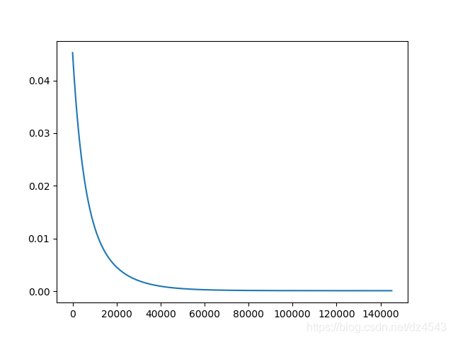
收敛时，得到的权重参数为：

array([0.31035205, 0.07770144, 0.21320657])

可以看到梯度下降得到的权重参数与直接求出法得出的基本相似，这其中的误差是因为没有进一步再迭代。

整合所有的代码如下：线性回归