Machine Learning-Programming Exercise 2: Logistic Regression

数据描述

前两列特征，第三列为输出的标签{0,1}

导入工具包


import numpy as np
import matplotlib
import matplotlib.pyplot as plt

读取文件函数


#将文本记录转化为Numpy
#filename为文件名，k为属性维数
def file2matrix(filename,k):
    fr = open(filename)
    numberOfLines = len(fr.readlines())         #get the number of lines in the file
    returnMat = np.zeros((numberOfLines,k))        #prepare matrix to return
    classLabelVector = np.zeros((numberOfLines,1))                #prepare labels return   
    fr = open(filename)
    index = 0
    for line in fr.readlines():
        line = line.strip()
        listFromLine = line.split(',')
        returnMat[index,:] = listFromLine[0:k]
        classLabelVector[index,:] = int(listFromLine[-1])
        index += 1
    return returnMat,classLabelVector

读取数据


#读取数据
returnMat, LabelVector = file2matrix('ex2data2.txt',2)

这里，returnMat是输入数据，LabelVector是输出标签(int 类型)，k为特征的数量。

对读取的数据可视化


#画图
pos = np.where(LabelVector == 1)[0]#正例
neg = np.where(LabelVector == 0)[0]#反例

fig = plt.figure()
ax = fig.add_subplot(111)
ax.scatter(returnMat[pos,0],returnMat[pos,1],c='y',marker='o')
ax.scatter(returnMat[neg,0],returnMat[neg,1],c='b',marker='x')
plt.xlabel('x1')
plt.ylabel('y1')
plt.show()

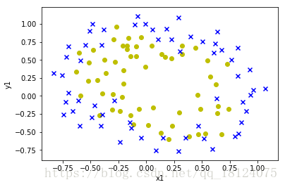
由上图可以知道，数据是非线性的。所以，需要对数据进行处理，具体处理方法见下面mapfeature。

Regularized Logistic Regression

这里如果不做正则化，只是单纯的Logistics Regression和作业1的程序一样，不同的是函数变为sigmoid。


def mapFeature(x1,x2):
    degree = 6
    out = np.ones((x1.shape[0],1))
    for i in range(1,degree+1,1):#产生1-degree的等差数列
        for j in range(0,i+1,1):
            out = np.column_stack((out,np.multiply(np.power(x1,i-j), (np.power(x2,j)))))#n次幂，点乘（矩阵乘法）
    return out

def sigmoid(z):
    g = 1/(1 + np.exp(-z))
    return g

def costFunctionReg(theta, X, y, lambda_value):
    m = y.shape[0]
    theta_1 = theta
    theta_1[0] = 0 #作为第一个常数的系数，应该去掉，不能参与正则化
    tmp1 = np.multiply(y,np.log(sigmoid(np.dot(X,theta))))
    tmp2 = np.multiply(1-y,np.log(1-sigmoid(np.dot(X,theta))))
    tmp3 = tmp1 + tmp1
    
    J = -1/m * np.sum(tmp3, axis=0) + lambda_value/(2*m)*np.dot(theta_1.T,theta_1)
    
    tmp4 = np.dot(X.T, sigmoid(np.dot(X,theta)) - y)
    grad = tmp4/m + lambda_value/m * theta_1
    return J, grad

特征映射


X = mapFeature(returnMat[:,0],returnMat[:,1])

由上图可以知道，x1和x2是的非线性的，所以需要将数据向高维映射。这里是将其转化为x1,x2,x1^2,x2^2,x1^2*x2,x2^2*x1,...。这里需要注意的是如果想更低维度的降维，只能让数据更加非线性。就好比浓缩是精华，是会让其更加的浓。而稀释之后可以减少浓度，使其变淡。

损失和梯度的计算


# Initialize fitting parameters
initial_theta = np.zeros((X.shape[1],1))

# Set regularization parameter lambda to 1
lambda_value = 1

# Compute and display initial cost and gradient for regularized logistic regression
J, grad = costFunctionReg(initial_theta, X, LabelVector, lambda_value)

print('Cost at initial theta (zeros): ', J[0][0])

这里，经过mapfeature变换之后，第一列是常数系数，全部为1，后面为变量系数。所以theta的维度也需要与mapfeature变换之后的结果保持对应。有吴恩达的讲义可以知道：

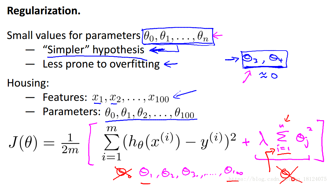
这里，我们需要注意的是在正则化的时候theta的常数项不参与计算，所以这里将其赋值给另外一个变量且常数项赋值为0。惩罚项的计算是将theta_1' * theta_1之后的结果，等价于图中的平方然后求和公式。

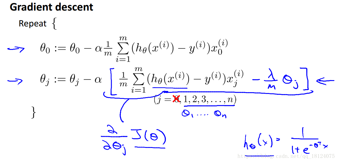
在计算grad的时候，需要两个公式是分开的，但是我们在前面将theta赋值给另外一个变量theta_1且theta_1常数项赋值为0。于是我们可以将两个公式合并为一个公式，在j = 0的时候，lambda / m * 0 = 0。

最后，数据和jupyter notebook下载处为https://download.csdn.net/download/qq_18124075/10529927。

Machine Learning-Programming Exercise 2: Logistic Regression

猜你喜欢