数据描述
数据:房屋面积+卧室个数+房价。其中,房屋面积和卧室个数位自变量,房价为因变量。数据下载链接
导入python包
import numpy as np
import matplotlib
import matplotlib.pyplot as plt
子函数描述
#将文本记录转化为Numpy
#filename为文件名,k为属性维数
def file2matrix(filename,k):
    fr = open(filename)
    numberOfLines = len(fr.readlines())         #get the number of lines in the file
    returnMat = np.zeros((numberOfLines,k))        #prepare matrix to return
    classLabelVector = np.zeros((numberOfLines,1))                #prepare labels return
    fr = open(filename)
    index = 0
    for line in fr.readlines():
        line = line.strip()
        listFromLine = line.split(',')
        returnMat[index,:] = listFromLine[0:k]
        classLabelVector[index,:] = float(listFromLine[-1])
        index += 1
    return returnMat,classLabelVector

#特征标准化
def featureNormalize(X):
    X_norm = np.array(X)
    #mu = np.zeros((1,X.shape[1]))
    #sigma = np.zeros((1, X.shape[1]))
    mu = np.mean(X, axis = 0)#对每列求均值
    sigma = np.std(X, axis = 0)#对每列求标准差
    X_norm = (X_norm - np.tile(mu, (X.shape[0],1)))/np.tile(sigma, (X.shape[0],1))
    return X_norm, mu, sigma

# 损失函数
def computeCostMulti(X, y, theta):
    m = len(y)
    J = np.sum((y - np.dot(X, theta))**2) / (2 * m)
    return J

#梯度下降
def gradientDescentMulti(X, y, theta, alpha, numb_iters):
    # Initialize some useful values
    m = len(y) # number of training examples
    J_history = []

    for i in range(numb_iters):
        theta -= alpha / m * np.dot(X.T, (np.dot(X, theta) - y))
        J_history.append(computeCostMulti(X, y, theta))
    return theta, J_history

# Normal Equation
# theta = (X'X)^(-1)X'y
def normalEqn(X, y):
    from numpy.linalg import inv
    return np.dot(np.dot(inv(np.dot(X.T, X)), X.T), y)
读入数据
returnMat, LabelVector = file2matrix('ex1data2.txt',2)
这里,我们对文件进行读取。首先,open文件并读取其行数,定义存放特征数据和预测数据的变量(这里,我们使用的类型是np.array。其实我们也可以使用np.mat,都是大同小异)。然后,利用strip移除字符串头尾指定的字符(默认为空格或换行符)或字符序列,利用split(',')指定分隔符(这里为',')对字符串进行切片,将前两列存入特征数据中,最后一列存入预测数据中。这里,如果预测数据是英文字母,我们还需要对其进行类型的转换。returnMat, LabelVector分别为存放特征数据和预测数据的变量。
特征标准化
# Part 1: Feature Normalization
X, mu, sigma = featureNormalize(returnMat)
我们对returnMat的数据求每一列的均值和标准差,这里使用到的函数为numpy自带的np.mean和np.std,具体使用详情可以查阅官方文件。然后使用np.tile对变量内容复制成输入矩阵同大小的矩阵。最后,(returnMat-mean)/std为标准化之后的结果,这里的‘/’是点除。
输入数据扩充
# Add intercept term to X
X = np.column_stack((np.ones((X.shape[0],1)), X))
我们在特征数据的第一列插入一列1矩阵,方便与之后delta的常数项系数相乘。
梯度下降
# Part 2: Gradient Descent
# Choose some alpha value
alpha = 0.01
num_iters = 400
# Init Theta and Run Gradient Descent
theta = np.zeros((X.shape[1],1))
theta, J_history = gradientDescentMulti(X, LabelVector, theta, alpha, num_iters)
梯度下降法的公式参见下图
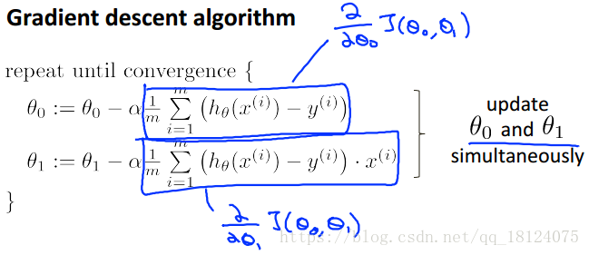
由公式可以知道,对于常数求偏导之后不会乘x。所以我们将x转置,第一列常数项全部为1,任何数乘以1都是其本身。而且利用x转置乘以误差项也可以达到将所有样例求和的目的。
theta -= alpha / m * np.dot(X.T, (np.dot(X, theta) - y))
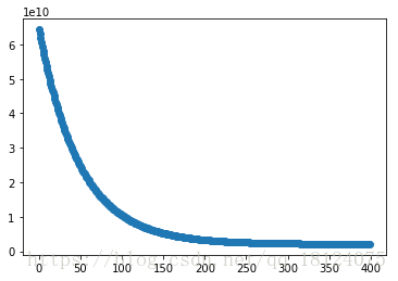
迭代误差结果图
fig = plt.figure()
ax = fig.add_subplot(111)
ax.scatter(range(len(J_history)), J_history)
plt.show()
预测
# 预测
# Estimate the price of a 1650 sq-ft, 3 br house
# Recall that the first column of X is all-ones. Thus, it does not need to be normalized.

price = np.dot(np.column_stack((np.array([[1]]), ((np.array([[1650, 3]]) - mu) / sigma))), theta)

print("Predicted price of a 1650 sq-ft, 3 br house is $", price[0][0])
结果:Predicted price of a 1650 sq-ft, 3 br house is $ 289221.547371
这里,我们需要注意的是数据刚开始就标准化,所以这里的数据也需要进行标准化。
Normal Equations
# Part 3: Normal Equations
X, y = file2matrix('ex1data2.txt',2)
# Add intercept term to X
X = np.column_stack((np.ones((X.shape[0],1)), X))
theta1 = normalEqn(X, LabelVector)


# 预测
# Estimate the price of a 1650 sq-ft, 3 br house
# Recall that the first column of X is all-ones. Thus, it does not need to be normalized.

price1 = np.dot(np.column_stack((np.array([[1]]), np.array([[1650, 3]]))), theta1)

print("Predicted price of a 1650 sq-ft, 3 br house is $", price1[0][0])
最小二乘法的delta用矩阵的形式表示为:
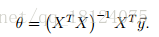
结果:Predicted price of a 1650 sq-ft, 3 br house is $ 293081.464335。这里,因为刚开始没有对数据进行标准化处理,所以在预测时候也不需要进行标准化处理。