Machine Learning Experiment4： Logistic Regression and Newton’s Method 详解+源代码解析

1. 回顾Logistic Regression的基本原理

1. 关于sigmoid函数

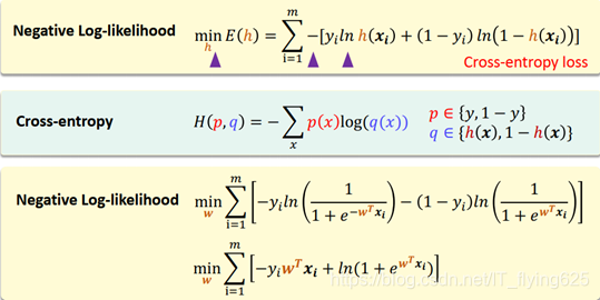
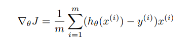
1. 极大似然与损失函数

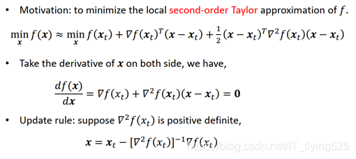
1. 牛顿法

1. 实验步骤与过程

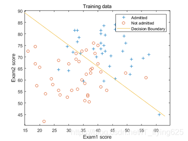
1. 首先，读入数据并绘制原始数据散点图

 

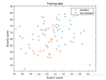
根据图像，我们可以看出，左下大多为负样本，而右上多为正样本，划分应该大致为一个斜率为负的直线。

1. 定义预测方程：

此处使用sigmoid函数，定义为匿名函数（因为在MATLAB中内联函数即将被淘汰）

1. 定义损失函数和迭代次数

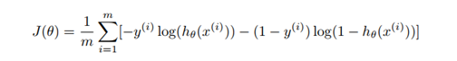
损失函数：

参数更新规则：

梯度：

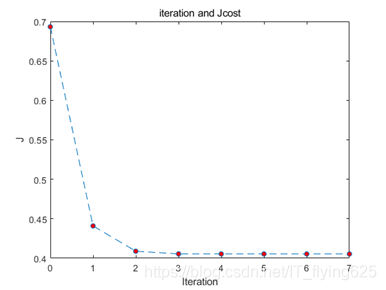
注意：其中，参数theta初始化为0，初始定义迭代次数为20，然后观察损失函数，调整到合适的迭代次数，发现当迭代次数达到6左右，就已经收敛。

1. 计算结果：通过迭代计算theta

theta = zeros(n+1, 1);  %theta 3x1

iteration=8

J = zeros(iteration, 1);

for i=1:iteration

    z = x*theta;   %列向量 80x1     x 80x3   y 80x1  

    J(i) =(1/m)*sum(-y.*log(g(z)) - (1-y).*log(1-g(z)));

    H = (1/m).*x'*(diag(g(z))*diag(g(-z))*x);%3x3  转换为对角矩阵

    delta=(1/m).*x' * (g(z)-y);

    theta=theta-H\delta

    %theta=theta-inv(H)*delta

end

计算得到的theta值为：

theta = 3×1

  -16.3787

    0.1483

    0.1589

绘制图像如下：

关于损失函数值与迭代次数的变化

预测：

预测成绩1为20，成绩二维80不被录取的概率：

prob = 1 - g([1, 20, 80]*theta)

计算得：

prob = 0.6680

即不被录取的概率为0.6680.

 

MATLAB源代码

clc,clear
x=load('ex4x.dat')
y=load('ex4y.dat')
[m, n] = size(x);
x = [ones(m, 1), x];%增加一列
% find returns the indices of the
% rows meeting the specified condition
pos = find(y == 1); neg = find(y == 0);
% Assume the features are in the 2nd and 3rd
% columns of x
plot(x(pos, 2), x(pos,3), '+'); hold on
plot(x(neg, 2), x(neg, 3), 'o')
xlim([15.0 65.0])
ylim([40.0 90.0])
xlim([14.8 64.8])
ylim([40.2 90.2])
legend({'Admitted','Not Admitted'})
xlabel('Exam1 score')
ylabel('Exam2 score')
title('Training data')
g=@(z)1.0./(1.0+exp(-z))
% Usage: To find the value of the sigmoid 
% evaluated at 2, call g(2)
theta = zeros(n+1, 1);  %theta 3x1
iteration=8
J = zeros(iteration, 1);
for i=1:iteration
    z = x*theta;   %列向量 80x1     x 80x3   y 80x1   
    J(i) =(1/m)*sum(-y.*log(g(z)) - (1-y).*log(1-g(z)));
    H = (1/m).*x'*(diag(g(z))*diag(g(-z))*x);%3x3  转换为对角矩阵
    delta=(1/m).*x' * (g(z)-y);
    theta=theta-H\delta
    %theta=theta-inv(H)*delta
end
% Plot Newton's method result
% Only need 2 points to define a line, so choose two endpoints
plot_x = [min(x(:,2))-2,  max(x(:,2))+2];
% Calculate the decision boundary line
plot_y = (-1./theta(3)).*(theta(2).*plot_x +theta(1));
plot(plot_x, plot_y)
legend('Admitted', 'Not admitted', 'Decision Boundary')
hold off
figure
plot(0:iteration-1, J, 'o--', 'MarkerFaceColor', 'r', 'MarkerSize', 5)
xlabel('Iteration'); ylabel('J')
xlim([0.00 7.00])
ylim([0.400 0.700])
title('iteration and Jcost')
prob = 1 - g([1, 20, 80]*theta)