[Machine Learning] Programming Exercise 1: Linear Regression

吴恩达机器学习课后作业。因为这学期内容不全，所以用的往年的题目。还未施工完成

第一章介绍了一下机器学习，监督学习，无监督学习，回归算法。
线性回归是一种有监督的学习，解决的是自变量和因变量之间的关系。
单变量线性回归就是从一个输入值预测一个输出值；而多变量线性回归就是从多个输入值预测一个输出值。
实验的目的在于学习单变量的线性回归和多变量线性回归算法，总之，以后看到线性的输入输出值关系，都可以带到下面的算法里面跑一下看看

单变量线性回归

第一步：实现代价函数
代价函数就是右边这个东东，

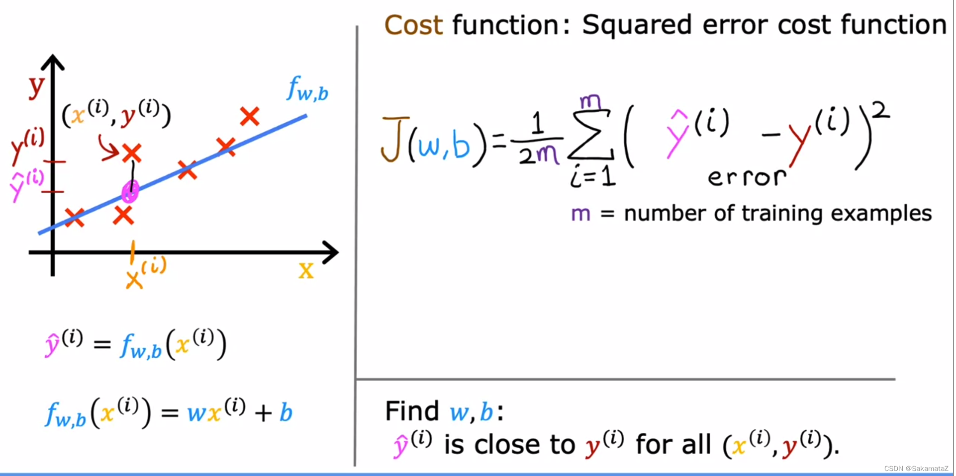
在线性回归中，我们假设数据呈线性分布，代价函数用于进行参数选择（即拟合），最常用的是最小均方误差函数

def computeCost(X,y,theta):
	m=len(X) 
	part=np.power((X*theta.T-y),2)
	return sum(part)/(2*m)

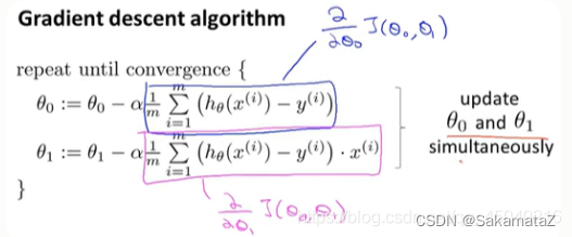
第二步：实现线性回归中的梯度下降函数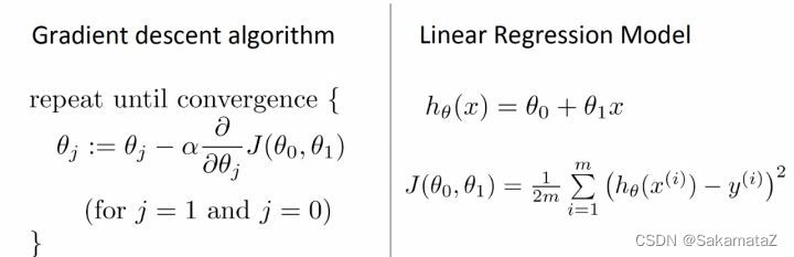

# theta是为0的初始矩阵，alpha是下降率，iters是梯度下降循环次数
def gradientDescent(X,y,theta,alpha,iters):
	temp=np.matrix(np.zeros(theta.shape))
	parameters=int(theta.ravel().shape[1])
	cost=np.zeros(iters)
	for i in range(iters): 
		error = (X*theta.T) - y 
		for j in range(parameters): 
			term=np.multiply(error,X[:,j])
			temp[0,j]=theta[0,j]-((alpha/len(X))*np.sum(term))
		theta=temp	
		cost[i]=computeCost(X,y,theta) 
	return theta,cost	

最后绘制线性模型，观察拟合程度。
完整代码如下：

import numpy as np
import pandas as pd
import matplotlib.pyplot as plt

def computeCost(X,y,theta):
	m = len(X) 
	inner = np.power(X*theta.T-y,2)
	return np.sum(inner)/(2*m)

def gradientDescent(X,y,theta,alpha,iters):
	temp = np.matrix(np.zeros(theta.shape))
	parameters = int(theta.shape[1])
	cost=np.zeros(iters)
	for i in range(iters):
		error = X*theta.T - y
		for j in range(parameters):
			term=np.multiply(error,X[:,j]) 
			temp[0,j]=temp[0,j] - (alpha*np.sum(term)/(len(X)))
		theta=temp
		cost[i]=computeCost(X,y,theta)
	return cost,theta

alpha = 0.01
iters = 1500
path = 'ex1data1.txt'
data = pd.read_csv(path,header=None,names=['Population','Profit'])

data.plot(kind='scatter',x='Population',y='Profit',figsize=(12,8))
plt.show()

data.insert(0,'Ones',1,False)
cols = data.shape[1]
X = data.iloc[:,:-1]
y = data.iloc[:,cols-1:cols]

X = np.matrix(X)
y = np.matrix(y)
theta = np.matrix(np.array([0,0]))


cost,theta=gradientDescent(X,y,theta,alpha,iters)
print(cost)
print(theta)

predict1=[1,3.5]*theta.T
predict2=[1,7]*theta.T
print(predict1)
print(predict2)

x = np.linspace(data.Population.min(),data.Population.max(),100)
f = theta[0,0] + (theta[0,1] * x)

fig,ax=plt.subplots(figsize=(12,8))
ax.plot(x,f,'r',label='Prediction')
ax.scatter(data.Population, data.Profit, label='Traning Data')
ax.legend(loc=2)
ax.set_xlabel('Population')
ax.set_ylabel('Profit')
ax.set_title('Predicted Profit vs. Population Size')
plt.show()

多变量线性回归

向量化和正规方程解决了多变量线性回归的问题

首先进行特征归一化：
特征归一化的目的是为了缩短梯度下降收敛的时间，提高速度。
特征归一化有两种常用的手段：1）最大最小规范化 2）Z-score均值规范化（如下图）

其次使用梯度下降法：

# 加一列常数项
data2.insert(0, 'Ones', 1)

# 初始化X和y
cols = data2.shape[1]
X2 = data2.iloc[:,0:cols-1]
y2 = data2.iloc[:,cols-1:cols]

# 转换成matrix格式，初始化theta
X2 = np.matrix(X2.values)
y2 = np.matrix(y2.values)
theta2 = np.matrix(np.array([0,0,0]))

# 运行梯度下降算法
g2, cost2 = gradientDescent(X2, y2, theta2, alpha, iters)
g2

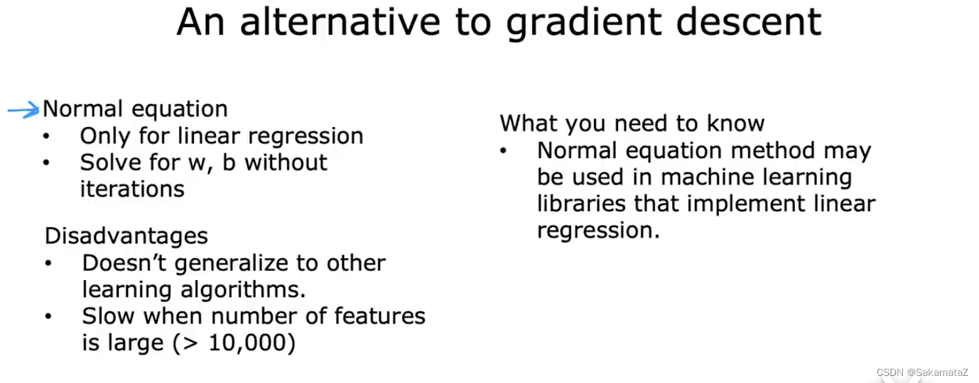
正规方程方法：
正规方程和梯度下降的区别，梯度下降需要迭代、耗费系统资源较多、需要选择学习率、适用性良好；正规方程法无需选择学习率、无需迭代计算、n很大的时候计算缓慢

def normalEqn(X,y):
	# A=np.linalg.inv(X.T*X)
	# theta=A*X.T*y
	theta = np.linalg.inv(X.T@X)@X.T@y#X.T@X等价于X.T.dot(X)
	return theta
final_theta2 = normalEqn(X,y)
print(final_theta2)