本文是基于吴恩达老师《深度学习》第二周第一课练习题所做,目的在于探究参数初始化对模型精度的影响。
一、数据处理
本文所用第三方库如下,其中reg_utils 和 testCases_regularization为辅助程序从这里下载。
import numpy as np
import matplotlib.pyplot as plt
from reg_utils import *
import sklearn
import sklearn.datasets
import scipy.io
from testCases_regularization import *
本次课程中使用了一个比较有趣的例子:使用人工智能的方法为一支足球队做技术分析,为队员预测头球破门率最高的位置。

下图给出了过去十场比赛中,该队与对手抢得头球点的数据集

蓝色点表示本队抢到头球时队员所在的位置,红点表示对手抢到头球时所在的位置。本文的任务是建立深层神经网络对该数据集进行训练,为了分析正则化对构建神经网络的作用,我们分别构建无正则化模型、L2正则化模型和dropout模型,并对三者的结果进行对比研究。
二、深层神经网络模型
在该文中已经详细说明过模型所用到的各函数的意义,再此不再赘述。
def model(X, Y, learning_rate = 0.3, num_iterations = 30000, print_cost = True, lambd = 0,keep_prob = 1):

    grads = {}
    costs = []
    m = X.shape[1]
    layers_dims = [X.shape[0], 20, 3, 1]

    parameters = initialize_parameters(layers_dims)

    for i in range(0, num_iterations):

        if keep_prob == 1:
            a3, cache = forward_propagation(X, parameters)

        elif keep_prob < 1:
            a3, cache = forward_propagation_with_dropout(X, parameters)

        if lambd == 0:
            cost = compute_cost(a3, Y)

        else:
            cost = compute_cost_with_regularization(a3, Y, parameters, lambd)

        assert(lambd == 0 or keep_prob == 1)

        if lambd == 0 and keep_prob == 1:
            grads = backward_propagation(X, Y, cache)

        elif lambd != 0:
            grads = backward_propagation_with_regularization(X, Y, cache, lambd)

        elif keep_prob < 1:
            grads = backward_propagation_with_dropout(X, Y, cache, keep_prob)

        parameters = update_parameters(parameters, grads, learning_rate)

        if print_cost == True and i % 10000 ==0:
            print("cost after iterations {}:{}".format(i,cost))
        if print_cost == True and i % 1000 ==0:
            costs.append(cost)

    plt.plot(costs)
    plt.xlabel("iterations (per 1000)")
    plt.ylabel("cost")
    plt.title("Learning rate = " + str(learning_rate))
    plt.show()

    return parameters
三、无正则化模型
我们先测试一下模型没有正则化和dropout优化的情况下,测试效果是怎样的
parameters = model(train_X, train_Y)
print("On the training set:")
predictions_train = predict(train_X, train_Y, parameters)
print("On the test set:")
predictions_test = predict(test_X, test_Y, parameters)
cost after iterations 0:0.6557412523481002
cost after iterations 10000:0.16329987525724213
cost after iterations 20000:0.13851642423245572
On the training set:
Accuracy: 0.9478672985781991
On the test set:
Accuracy: 0.915
在训练集和测试集上的预测精度分别是94.78%,91.5%,训练集上精度比测试集高3%,看起来有些过拟合,我们打印出边界曲线看下效果。

图中可以明显看出,对于测试集确实有些过拟合,下面我们使用L2正则化和dropout方法,看看如何改善过拟合现象。
四、L2正则化模型
L2范数在神经网络中也成为F范数(弗罗贝尼乌斯范数),在使用L2正则化的同时,cost函数也需要进行相应的修改。

def compute_cost_with_regularization(A3, Y, parameters, lambd):
    m = Y.shape[1]
    W1 = parameters["W1"]
    W2 = parameters["W2"]
    W3 = parameters["W3"]

    cross_entropy_cost = compute_cost(A3, Y)

    L2_regularization_cost = (1. / m * lambd / 2) * (np.sum(np.square(W1))+
                                                     np.sum(np.square(W2))+
                                                     np.sum(np.square(W3)))
    cost = cross_entropy_cost + L2_regularization_cost

return costdef backward_propagation_with_regularization(X, Y, cache, lambd):
m = X.shape[1]
(Z1, A1, W1, b1,Z2, A2, W2, b2,Z3, A3, W3, b3) = cache
dZ3 = A3 - Y
dW3 = 1. / m * np.dot(dZ3, A2.T) + lambd / m * W3
db3 = 1. / m * np.sum(dZ3, axis=1, keepdims = True)
dA2 = np.dot(W3.T, dZ3)
dZ2 = np.multiply(dA2, np.int64(A2>0))
dW2 = 1. / m * np.dot(dZ2, A1.T) + lambd / m * W2
db2 = 1. / m * np.sum(dZ2, axis=1, keepdims = True)
dA1 = np.dot(W2.T, dZ2)
dZ1 = np.multiply(dA1, np.int64(A1>0))
dW1 = 1. / m * np.dot(dZ1, X.T) + lambd / m * W1
db1 = 1. / m * np.sum(dZ1, axis=1, keepdims = True)
gradients = {"dZ3": dZ3, "dW3": dW3, "db3": db3,"dA2": dA2,
"dZ2": dZ2, "dW2": dW2, "db2": db2, "dA1": dA1,
"dZ1": dZ1, "dW1": dW1, "db1": db1}
return gradients
我们设lambd = 0.7,运行模型观察预测效果:
cost after iterations 0:0.6974484493131264
cost after iterations 10000:0.26849188732822393
cost after iterations 20000:0.2680916337127301
parameters = model(train_X, train_Y, lambd = 0.7)
print("On the training set:")
predictions_train = predict(train_X, train_Y, parameters)
print("On the test set:")
predictions_test = predict(test_X, test_Y, parameters)
On the training set:
Accuracy: 0.9383886255924171
On the test set:
Accuracy: 0.93
此时增加L2正则化后,训练集和测试集的预测精度分别是93.8%和93%
plt.title("Model with L2-regularization")
axes = plt.gca()
axes.set_xlim([-0.75,0.40])
axes.set_ylim([-0.75,0.65])
plot_decision_boundary(lambda x : predict_dec(parameters, x.T),train_X, train_Y)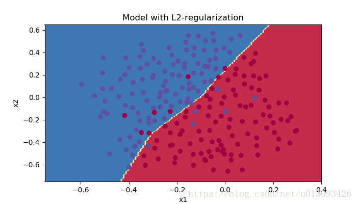
过拟合现象大大改善。
五、dropout模型
dropout的基本原理在每层网络上随即的让一些神经元失活,这样使得网络模型更加简化,可以改善过拟合现象。dropout作用的网络层通常是W比较复杂的,对于只有少数神经元的层次则不需要作用。增加dropout算法后,前向传播和反向传播的过程都会受到影响。
(1)前向传播
def forward_propagation_with_dropout(X, parameters, keep_prob=0.5):
    np.random.seed(1)

    W1 = parameters["W1"]
    b1 = parameters["b1"]
    W2 = parameters["W2"]
    b2 = parameters["b2"]
    W3 = parameters["W3"]
    b3 = parameters["b3"]

    Z1 = np.dot(W1,X) + b1
    A1 = relu(Z1)
    D1 = np.random.rand(A1.shape[0], A1.shape[1])
    D1 = D1 < keep_prob
    A1 = A1 * D1
    A1 = A1 / keep_prob

    Z2 = np.dot(W2, A1) + b2
    A2 = relu(Z2)
    D2 = np.random.rand(A2.shape[0], A2.shape[1])
    D2 = D2 < keep_prob
    A2 = A2 * D2
    A2 = A2 / keep_prob

    Z3 = np.dot(W3, A2) + b3
    A3 = sigmoid(Z3)

    cache = (Z1, D1, A1, W1, b1, Z2, D2, A2, W2, b2, Z3, A3, W3, b3)

    return A3, cache
(2)反向传播
def backward_propagation_with_dropout(X, Y, cache, keep_prob):
    m = X.shape[1]
    (Z1, D1, A1, W1, b1, Z2, D2, A2, W2, b2, Z3, A3, W3, b3) = cache

    dZ3 = A3 - Y
    dW3 = 1. / m * np.dot(dZ3, A2.T)
    db3 = 1./ m * np.sum(dZ3, axis = 1, keepdims = True)

    dA2 = np.dot(W3.T, dZ3)
    dA2 = dA2 * D2
    dA2 = dA2 / keep_prob
    dZ2 = np.multiply(dA2, np.int64(A2>0))
    dW2 = 1. / m * np.dot(dZ2, A1.T)
    db2 = 1. / m * np.sum(dZ2, axis=1, keepdims = True)

    dA1 = np.dot(W2.T, dZ2)
    dA1 = dA1 * D1
    dA1 = dA1 / keep_prob
    dZ1 = np.multiply(dA1, np.int64(A1>0))
    dW1 = 1. / m * np.dot(dZ1, X.T)
    db1 = 1. / m * np.sum(dZ1, axis = 1, keepdims = True)

    gradients = {"dZ3": dZ3, "dW3": dW3, "db3": db3,"dA2": dA2,
                 "dZ2": dZ2, "dW2": dW2, "db2": db2, "dA1": dA1,
                 "dZ1": dZ1, "dW1": dW1, "db1": db1}

    return gradients
我们给定Keep_prob为0.86,即以24%的概率失活各层神经元,调用模型如下
parameters = model(train_X, train_Y, keep_prob = 0.86, )
print("On the training set:")
predictions_train = predict(train_X, train_Y, parameters)
print("On the test set:")
predictions_test = predict(test_X, test_Y, parameters)
cost after iterations 0:0.6543912405149825
cost after iterations 10000:0.0610169865749056
cost after iterations 20000:0.060582435798513114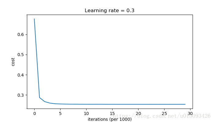
On the train set:
Accuracy: 0.9289099526066351
On the test set:
Accuracy: 0.95
该方法在训练集和测试集上的预测精度分别是92.89%和95,在训练集上的预测效果更有,过拟合问题得到了很好的解决。
plt.title("Model with dropout")
axes = plt.gca()
axes.set_xlim([-0.75,0.40])
axes.set_ylim([-0.75,0.65])
plot_decision_boundary(lambda x: predict_dec(parameters, x.T), train_X, train_Y)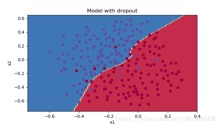
六、总结
正则化可以很好的解决模型过拟合的问题,常见的正则化方式有L2正则化和dropout,但是正则化是以牺牲模型的拟合能力来达到平衡的,因此在对训练集的拟合中有所损失。