【机器学习课程-华盛顿大学】：1 案例研究 1.2 回归（2）房价预测实战

房价预测实战

1、加载库和数据

import graphlab
graphlab.set_runtime_config('GRAPHLAB_DEFAULT_NUM_PYLAMBDA_WORKERS', 4)

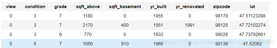
sales = graphlab.SFrame('home_data.gl/')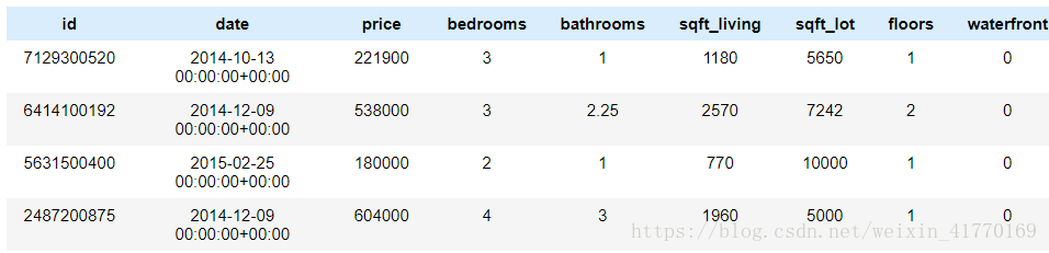

2、数据集、测试集分割

train_data,test_data = sales.random_split(.8,seed=0)

3、2元线性回归预测

（1）特征：sqft_living, 预测结果：price

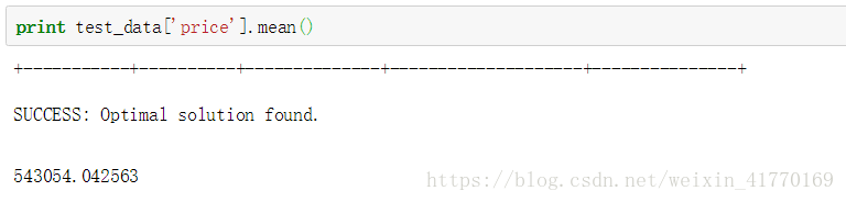
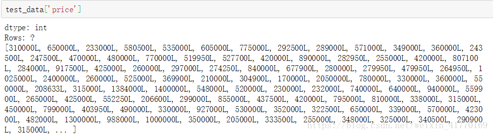
sqft_model = graphlab.linear_regression.create(train_data, target='price', features=['sqft_living'],validation_set=None)

（2）测试：

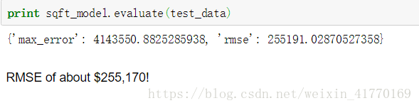
（3）可视化

import matplotlib.pyplot as plt
%matplotlib inline

plt.plot(test_data['sqft_living'],test_data['price'],'.',
        test_data['sqft_living'],sqft_model.predict(test_data),'-')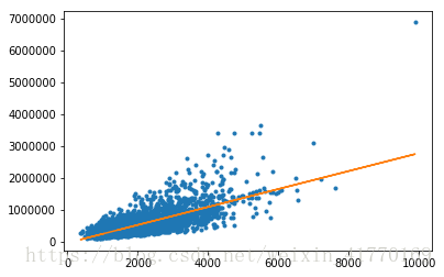

sqft_model.get('coefficients')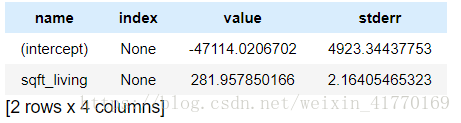

4、多元线性回归预测

（1）特征：6个，预测结果：price

my_features_model = graphlab.linear_regression.create(train_data,target='price',features=my_features,validation_set=None)

（2）比较二元、多元线性预测结果

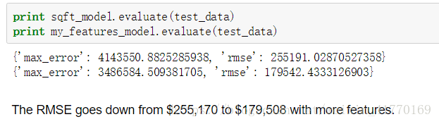
5、测试

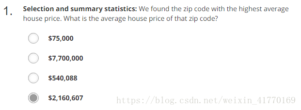
sales[sales['zipcode']=='98039']['price'].mean()

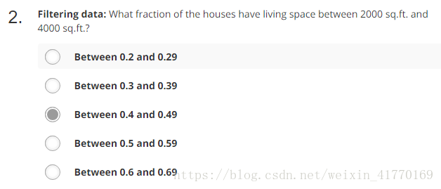
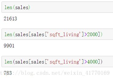
(9901-783)/21613 = 0.42