Python机器学习实战1:使用线性回归模型来解决波士顿房价预测和研究生入学率问题

boston房价预测
导入库
from  sklearn.linear_model import LinearRegression
from  sklearn.datasets import load_boston
import matplotlib.pyplot as plt
%matplotlib inline
获取数据集
bosten = load_boston()
线性回归
- 模型训练
clf = LinearRegression()
clf.fit(bosten.data[:,5:6],bosten.target)  #模型训练
x = bosten.data[:,5:6]
- 回归系数
clf.coef_
array([9.10210898])
- 预测值
y_pre = clf.predict(bosten.data[:,5:6]) #模型的输出值
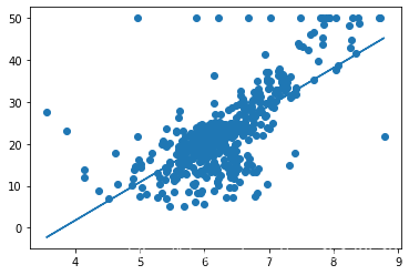
- 可视化
plt.scatter(x,bosten.target)
plt.plot(x,y_pre)
plt.show()
研究生入学率
导入库
import pandas as pd
from sklearn.linear_model import LogisticRegression  #逻辑回归
from sklearn.model_selection import train_test_split  #测试集训练集分割
from sklearn.metrics import classification_report
导入数据
data = pd.read_csv(r"LogisticRegression.csv")
data_tr,data_te,label_tr,label_te = train_test_split(data.iloc[:,1:],data["admit"],test_size = 0.2)
data.iloc[:,1:]
| gre | gpa | rank | |
|---|---|---|---|
| 0 | 380 | 3.61 | 3 |
| 1 | 660 | 3.67 | 3 |
| 2 | 800 | 4.00 | 1 |
| 3 | 640 | 3.19 | 4 |
| 4 | 520 | 2.93 | 4 |
| ... | ... | ... | ... |
| 395 | 620 | 4.00 | 2 |
| 396 | 560 | 3.04 | 3 |
| 397 | 460 | 2.63 | 2 |
| 398 | 700 | 3.65 | 2 |
| 399 | 600 | 3.89 | 3 |
400 rows × 3 columns
data_tr.head()
| gre | gpa | rank | |
|---|---|---|---|
| 252 | 520 | 4.00 | 2 |
| 94 | 660 | 3.44 | 2 |
| 41 | 580 | 3.32 | 2 |
| 2 | 800 | 4.00 | 1 |
| 207 | 640 | 3.63 | 1 |
data_te.head()
| gre | gpa | rank | |
|---|---|---|---|
| 45 | 460 | 3.45 | 3 |
| 311 | 660 | 3.67 | 2 |
| 391 | 660 | 3.88 | 2 |
| 357 | 720 | 3.31 | 1 |
| 117 | 700 | 3.72 | 2 |
模型训练
clf = LogisticRegression()
clf.fit(data_tr,label_tr)  #模型训练
pre = clf.predict(data_te) #模型预测
- 预测出来的标签,label_te实际值
pre
array([0, 0, 0, 1, 0, 0, 1, 1, 0, 0, 0, 0, 0, 0, 0, 0, 0, 0, 0, 0, 0, 0,
       0, 0, 0, 0, 0, 0, 0, 0, 1, 0, 0, 0, 0, 0, 0, 0, 0, 0, 0, 0, 0, 0,
       0, 0, 0, 1, 1, 0, 1, 0, 0, 0, 1, 0, 0, 0, 0, 0, 1, 0, 0, 0, 1, 0,
       0, 0, 0, 0, 0, 0, 0, 0, 0, 0, 0, 0, 0, 0], dtype=int64)
- sklearn中的classification_report函数用于显示主要分类指标的文本报告.在报告中显示每个类的精确度,召回率,F1值等信息。
res = classification_report(label_te,pre)
print(res)
              precision    recall  f1-score   support

           0       0.71      0.89      0.79        56
           1       0.40      0.17      0.24        24

    accuracy                           0.68        80
   macro avg       0.56      0.53      0.51        80
weighted avg       0.62      0.68      0.63        80
推荐阅读
到这里就结束了,如果对你有帮助你,欢迎点赞关注,你的点赞对我很重要